Before starting
Ask questions!!!!

About the computing methods in mathematics.
Numeric |
Symbolic |
|---|---|
| fast | usually slower |
| approximate | exact |
| well suited for simulations/DE/root finding | well suited for algebraic/geometric problems |
| sensible to unstability | always stable |
| not certified | certified |
| bertini/PHCpack... | CoCoA/Singular/Macaulay/Magma... |
| not good for exact problems | hopeless for certain problems |
Motivation
Let $C = V(f), f\in \mathbb{C}[x,y]$ be a plane affine curve. We are interested in the topology of the pair $(\mathbb{C}^2, C)$.
This has several ingredients:
- The topology of the ambient space $\mathbb{C}^2$ is easy (just $\mathbb{R}^4$).
- The topology of the curve $C$ can be seen as a Riemann surface.
So the complexity lies on the embedding. In particular, we will focus on the complement $\mathbb{C}^2\setminus C$. Its main invariant is the fundamental group.


Theorem (Zariski-Van Kampen)
The fundamental group $\pi_1(\mathbb{C}^2\setminus C)$ is given by the quotient of the free group $F_d$ by the action of the braid monodromy.
Theorem (Moishezon, Carmona, Isaza...)
The topology of the pair is determined by the braid monodromy.
So our problem can be reduced to compute the braids corresponding to the loops around the points of the discriminant.
Definition:
Two curves $C_1= V(f_1), C_2=V(f_2)$ form a weak arithmetic Zariski pair if these two conditions hold:
- $f_1$ and $f_2$ are Galois conjugate.
- $(\mathbb{C}^2, C_1)$ and $(\mathbb{C}^2, C_2)$ are not homeomorphic.
There exist weak arithmetic Zariski pairs. In particular it means that we cannot use only algebraic methods to study the embedded topology.
But maybe there is hope for the fundamental group:
Lemma:
$\pi_1^{alg}(\mathbb{C}^2\setminus C)$ is isomorphic to the profinite completion of $\pi_1(\mathbb{C}^2\setminus C)$.
Nope:
Definition:
Two curves $C_1= V(f_1), C_2=V(f_2)$ form an arithmetic Zariski pair if:
- $f_1$ and $f_2$ are Galois conjugate.
- $\pi_1(\mathbb{C}^2\setminus C_1)$ and $\pi_1(\mathbb{C}^2\setminus C_1)$ are not isomorphic.
There exist arithmetic Zariski pairs. So we cannot use purely algebraic methods to compute the fundamental group either.
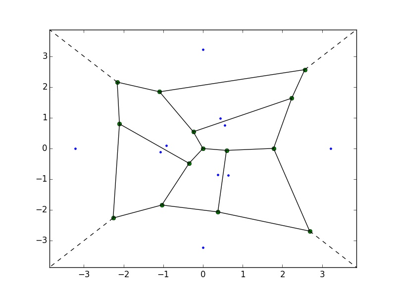
How to compute the braids
The paths in the base plane can be given by the Voronoi diagram of the discriminant.
How to compute the braids
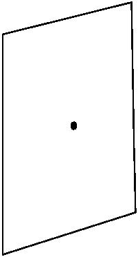
The problem can be reduced to compute the crossings of a braid over a segment. Without loss of generality, we can assume it goes from $0$ to $1$.
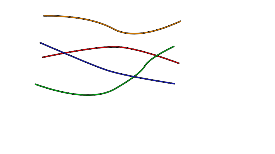
How to compute the braids
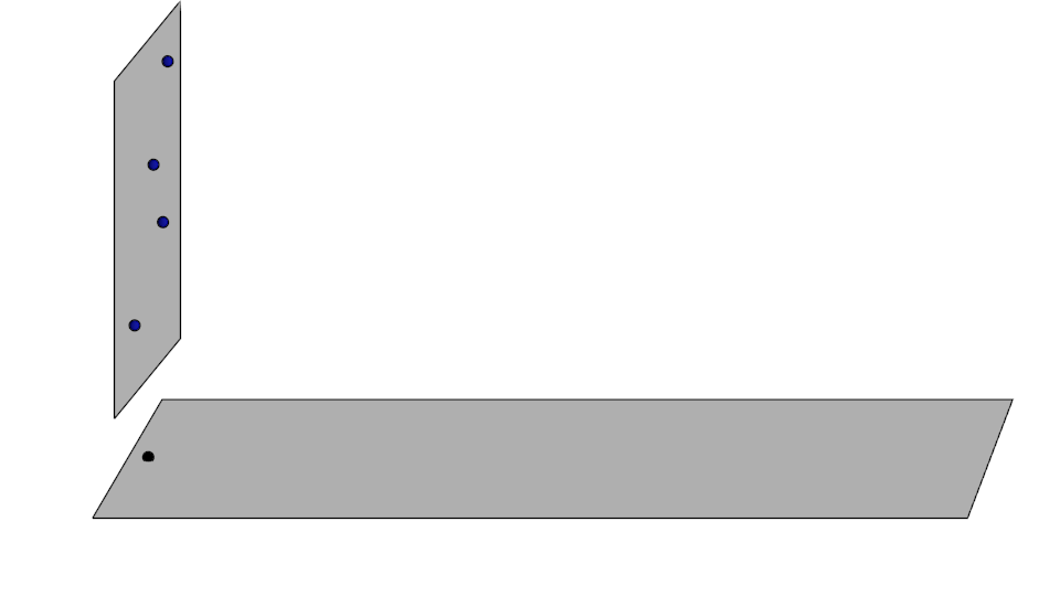
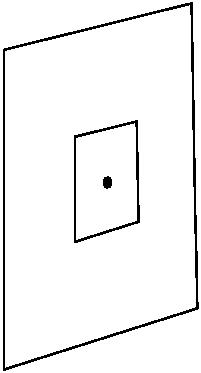
The idea is to aproximate the braid with a piecewise linear one. In order to do that we have to find aproximate roots and continue them.
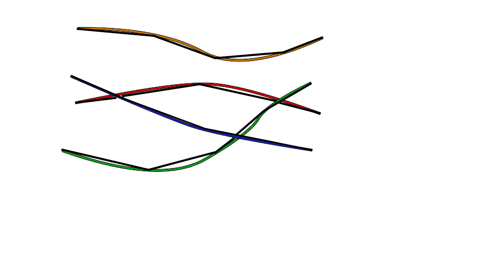
How to compute the braids
But we need to ensure that it is topologically correct. That is, that we don't miss any crossing, or jump from one strand to another.
Why not leverage existing solutions (Bertini, PHC...)?
- Only care about the final result (we need the intermediate steps)
- Non-certified (or certified in a weaker sense)
- License issues
- Specific methods for this dimension.
- Better performance.
The "ring" of real intervals
$\mathbb{R}_{int} := \{[a,b] \mid a,b \in\mathbb{R}, a\leq b\}$
- $[a_1, b_1] + [a_2,b_2] = [a_1+a_2,b_1+b_2]$
- $[a_1, b_1] \cdot [a_2,b_2] = \{x\cdot y \mid x\in[a_1,b_1], y\in [a_2,b_2]\}$
Pseudoinverses:
- $-[a,b] = [-b, -a]$
- $[a,b] ^{-1} = [b^{-1},a^{-1}]$ if $0\notin [a,b]$
The "ring" of complex intervals
$\mathbb{C}_{int} := \{A + i\cdot B \mid A, B \in \mathbb{R}_{int}\}$
$$[X] = \bigcap_{X\subseteq Y \in \mathbb{C}_{int}} Y$$- $(A_1+i\cdot B_1)+(A_2+i\cdot B_2) =[\{z_1+z_2 \mid z_i\in A_i+\cdot B_i\}] $
- $(A_1+i\cdot B_1)\cdot(A_2+i\cdot B_2) =[\{z_1\cdot z_2 \mid z_i\in A_i+i\cdot B_i \}] $
Theorem:
Let $Y\in\mathbb{C}_{int}, y_0 \in Y$. Let $f:Y\to \mathbb{C}$ be a holomorphic function. Assume that $0 \notin [f'(Y)]$, and
$$N(f, y_0, Y):= y_0-\frac{f(y_0)}{[f'(Y)]} \subseteq Y.$$Then there exists a unique zero of $f$ in $Y$. Moreover, this zero lives in $N(f,y_0,Y)$
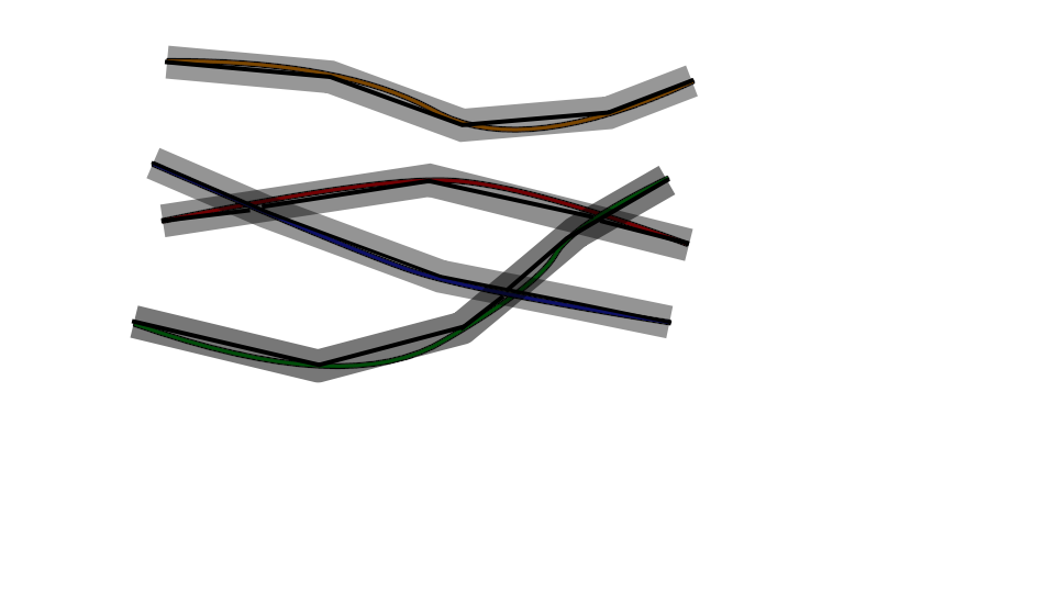
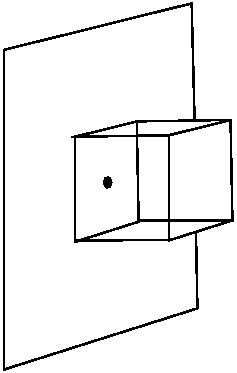
We can use this theorem to ensure that we have a tubular neighborhood of our piecewise linear braid that contains the actual braid.
Example:
$$f=[0.9, 1.1]\cdot y^2-1-x$$$$y_0 = 1$$$$Y = [0.5, 1.5]$$$$ x_0 = 0$$note that using intervals allows us to compute with irrational numbers, even transcendental!
Example: (extend x to an interval):
$$f=[0.9, 1.1]\cdot y^2-1-x$$$$y_0 = 1$$$$Y = [0.5, 1.5]$$$$ x = [0,0.25]$$So the braid will lie inside the interval around $y_0$ for $x \in [0,0.25]$.
Trick: change of variables

Trick: change of variables

Trick: change of variables

Trick: change of variables

Trick: change of variables

Trick: change of variables

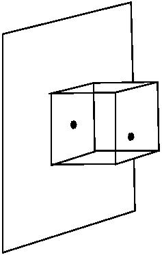
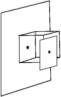
Double tubular neighborhood

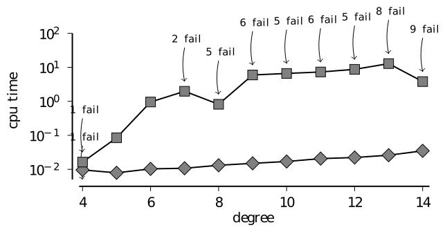
Timings and comparison
Demo:
load("sage-sirocco_interface.pyx")
load("ZVK.py")
R.<x,y> = QQ[]
f = x^2 + y^2 - 2
followstrand(f, 0, 1, 1.41)
f = y^3 - x
% time followstrand(f, 1, I, 1)
f = y^2 - x^3 - x^2
implicit_plot(f, (x, -3, 3), (y, -3, 3))

fundamental_group(f)
f = (x^2+y^2)^2+18*(x^2+y^2) - 27 -8*(x^3-3*x*y^2)
implicit_plot(f,(x,-3,3), (y,-3,3))

fundamental_group(f)
a = QQ[x](x^5-1).roots(QQbar)[-1][0]
a
F = NumberField(a.minpoly(), 'a', embedding = a)
F.inject_variables()
F
R.<x,y> = F[]
f = x^4 + a*y^4  - 2*x^2*y^2
fundamental_group(f)
R.<x,y> = QQ[]
f = -256*x^2*y^4 + 704*x*y^5 + 16*y^6 + 2048*x^3*y^2 - 6656*x^2*y^3 + 1872*x*y^4 + 36*y^5 - 4096*x^4 + 15360*x^3*y - 6528*x^2*y^2 + 2016*x*y^3 + 27*y^4 - 8960*x^3 + 576*x^2*y + 648*x*y^2 + 3888*x^2

implicit_plot(f,(x,-3,3),(y,-3,3))

%time G = fundamental_group(f, projective=True)
G