{
"cells": [
{
"cell_type": "markdown",
"metadata": {},
"source": [
"---\n",
"Infinity and Effectiveness from a Functional Point of View\n",
"\n",
"\n",
"By [*Francis Sergeraert*](https://www-fourier.ujf-grenoble.fr/~sergerar/Papers/Images.pdf), Published in the French journal *Images des Mathématiques*, 1990, vol.76, pp. 71 - 81.\n",
"\n",
"(Translation by Gerd Heber and [Google Translate](https://translate.google.com/), 16 April 2017.)\n",
"\n",
"---\n",
"\n",
"# Introduction\n",
"\n",
"*Infinity* and *effectiveness* are two concepts which seem to belong to two very distinct worlds. Is it possible to think of *infinity* in terms of *effectiveness*? The infinite is an *abstract* notion and thus appears beyond the reach of any *effective* approach, by which we mean one that can be translated into a concrete reality. Against this superficial impression, in this article, we will argue that effectiveness does not have to be sacrificed at the outset of an undertaking in which the infinite plays an essential role. This pursuit leads to many questions - and answers (!) - and is very exciting indeed.\n",
"\n",
"Mathematicians' ability to deal effectively with problems in which the infinite plays, in one form or another, an essential role, intimidates some and has earned them an air of sorcery. It can't be denied that this prowess has its place among the finest human achievements. The fame of several mathematicians can be attached directly to how they advanced our understanding of the infinite: Leibniz and Newton (infinitesimal calculus), Cantor (infinite sets), Cauchy (infinitesimal analysis), Hilbert (spaces of infinite dimension), Gödel (incompleteness), Robinson (non-standard analysis).\n",
"\n",
"Compared to the world of his mathematician colleague, superficial reflection might suggest that the computer scientist lives in a world more peaceful and less esoteric. The computer scientist works with machines (concrete or theoretical) that are in essence *finite*. Such machines can only work with programs, represented as *finite* texts, over necessarily *finite* data, for a *finite* time. But this view is not correct, and it is so for a variety of reasons. Perhaps the simplest reason is to point out that infinity is not studied by mathematicians for pleasure alone, but also because, very often, it is a powerful modeling tool. An example that immediately comes to mind is a numerical calculation: note that without an error estimation it is generally of little interest. However, most of the time such an estimation can only be done conveniently by means of differential calculus or the use of the *infinitely small*. On the (opposite) side, the infinitely large, we can point, for example, to the studies of algorithmic complexity, whose practical interest goes without saying and that are often based on asymptotic methods.\n",
"\n",
"In this article, we want to study a link between infinity and programming of an entirely different nature, the *functional* link. It is a rather subtle link, the description of which, however, is of extraordinary simplicity. It is so extraordinary that there is no reason to beat around the bush; let us describe it at once.\n",
"\n",
"A program is a finite object. In a specific instance, it will be represented by a piece of text, which is nothing but a finite sequence of characters, drawn from a finite alphabet, possibly the set of ASCII characters. Such a program may work on some given data (input) and retrun a result (output). Take for example a program $P$ that computes the square of a positive integer. It is capable of working on *every* integer $n\\in\\mathbb{N}$, and we immediately have our link: $P$ is finite while the set $\\mathbb{N}$ of the integers on which $P$ can work is not. In general, if $P$ is a program, let $I(P)$ ($I$ for *input*) denote the set of data on which it can work. The program $P$ is inherently finite whereas $I(P)$ can very well be infinite.\n",
"\n",
"Thus, by this sleight of hand, we've brought together the finite universe of ordinary objects with the mathematicians' realm, a people used to \"infinite monsters.\" It may seem that this is a mere philosophical consideration and without real interest. The purpose of this article is to convince you otherwise.\n",
"\n",
"It is organized as follows. We begin with the elementary example of a good program for calculating the chromatic number of a graph, which is well known to graph theorists and uses the functional point of view. It will be carefully described in order to isolate and highlight the problems of programming and *effectiveness* that are encountered in this kind of situation. It is hoped that the nature of the method and the difficulties to be anticipated will be well understood. It will then be time to examine the state of computer science in this matter. We will see that it is quite excellent: today's computer scientists have just what we need (lambda-calculus, functional languages) so that we can work on these issues in the best conditions. The machine construction of the *loop-space* functor, which is very easy to describe, will give a good example of the available programming capabilities. Once the right viewpoint is adopted and the right tools are available, rather simple programs, which require no more than student-level skills, can be used to build highly infinite spaces, in a blink of an eye, *on a machine*. These spaces are convenient to impress the galleries, but they do not serve only that: although infinite, Jean-Pierre Serre invented them around 1950 to solve problems of a *finite* nature (homotopy groups of spheres). We have similar intentions. In the last section, we will give the reader an idea of the substantial theoretical results already obtained in algebraic topology and a description of the beautiful field of work now open to programming to all who want to apply these methods concretely on a machine.\n",
"\n",
"Section 2 gives readers not accustomed to computer science a more precise description of the possibly infinite nature of the set $I(P)$.\n",
"\n",
"The basic approach to infinity using the functional method has often been used: Cauchy's approach to infinitesimal analysis is of this kind and is the subject of section 3.\n",
"\n",
"# Concerning the non-finiteness of the input set.\n",
"\n",
"In the introduction, we have considered the program $P$ which assigns to an integer $n$ its square $n^2$. Thus, if the program $P$ were presented with the integer 97, it should return 9409. To write such a program is straightforward in any language, for example on a calculator programmable in Basic.\n",
"\n",
"We denote by $I(P)$ the set of data that the program $P$ accepts as inputs. In the example of the square calculation, the set $I(P)$ is the set $\\mathbb{N}$ of the integers, which is known to be infinite.\n",
"\n",
"This statement might raise the suspicion of a reader who is used to doing practical work on a computer. The assertion that the set $I(P)$ is infinite may indeed suggest that its author is unaware of the real constraints in the use of such machines. On a Basic calculator, for example, an *integer* can only be used if it is smaller than a certain integer defined by the engineer who conceived this calculator. Often it is something like $2^{31}$ or $10^{10}$, so that the number of integers on which our example program is *actually* capable of working is really finite, and our critic is in the right. And this kind of constraint is present in most programming languages.\n",
"\n",
"This difficulty, however, can be circumvented by programs known to work in *multiprecision*. These programs use the following technique: Suppose that our machine only accepts integers smaller than $10^{10}$. Let us call an integer smaller than $b = 10^5$ ($b$ for base) a *small integer*. If $n$ is an arbitrary integer, we can always write it, and moreover in only one way, in the form $n = a_pb^p + a_{p-1}b^{p-1} + \\ldots + a_0$, where the $a_i$ are small integers. This amounts to cutting the decimal notation of $n$ into five-digit slices. It is also the base $b = 10^5$ notation of $n$. It is then easy to see that the analogous notation of the square $n^2$ of $n$ can be determined by means of a succession of operations on small integers alone, and hence on our calculator. Technically, we will represent $n$ as an *array* of small integers and the result $n^2$ will come out in a similar form. The rest is technique of index manipulations, elementary operations on small integers and carried numbers.\n",
"\n",
"It is thus possible, even on a modest calculator, to calculate the square of quite substantial integers, including ones with hundreds of digits. What has just been described was invented long ago by our ancestors, when they understood the surprising possibilities of writing numbers in any base, 10 for example. They realized that the same method, or shall we say *program*, can be used to multiply two integers admitting *any* number of digits! It is strictly the same phenomenon that has just been described, except that the base is $10^5$ instead of $10$, but this does not change the case. And it is thanks to this that the usual multiplication table does not need to go beyond $9\\times 9 = 81$. Multiprecision computing software is now becoming more widespread. It is even integrated in some languages (Lisp) and can be found in most formal computational systems.\n",
"\n",
"But our astute critic might try another argument. Of course, we are now able to multiply arbitrarily large integers, but there remains a limitation, that of the amount of available memory in the machine. The critic is right. If, for example, each small integer occupies a memory cell, then the largest integer that can be *stored* in the machine in an array of small integers will be $N = 10^{5M}-1$, where $M$ is the number of available memory cells. If an integer is greater than $N$, it is impossible to enter it in the machine and a fortiori to calculate the square.\n",
"\n",
"However, this limitation can be overcome by *expandable memory* machines, which can carry out the following operations. In a first step, a program is written, for example, a program that works on multiprecision integers. Then the program is called upon to perform a certain task. It is then possible to determine the amount of memory needed *for this particular use*. If need be, the memory can be extended before the computation gets underway. We see that, *in this sense*, our program can work on any integer.\n",
"\n",
"The critic may shrug his shoulders one last time: If the number of memory cells required for a calculation is greater than the number of atoms of our galaxy, it is going to be a long wait for the necessary memory extensions, which would be already difficult for much smaller extensions. Be that as it may, the theoretician is satisfied with this fact: *potentially* his program is able to work on an integer of any size.\n",
"\n",
"The term *theorist*, which has just been used, is sometimes a little pejorative: the appellation of theorist often designates a person especially incapable of practical realizations! In this article, we will convince the reader that these theoretical considerations of programs with potential infinities are, on the contrary, capable of quite concrete applications! Since we speak here of theory, we cannot fail to recall that this type of an extensible memory machine was perfectly modeled by the English mathematician Turing, well before the very existence of the word *computer*. Turing had invented his model to respond negatively to Hilbert's conjecture of a universal algorithm for solving mathematical problems. Knowing that Turing's work played an essential role in the genesis of modern computing, we have a good argument to use against those who still have doubts about the interest of fundamental research. For more on these questions, we highly recommoned *\"Allen Turing, the enigma\"* by Andrew Hodges (Simon & Schuster, 1983). A French translation was published in 1987 under the title *\"Alan Turing ou l'énigme de l'intelligence\"* at the Bibliothèque Scientifique Payot.\n",
"\n",
"# The Cauchy solution for infinitesimal analysis.\n",
"\n",
"The *functional trick*, an application which is the topic of this article, has been known for a long time. It is, for example, the essential tool of the modern formalization of the infinitesimal analysis, usually attributed to Cauchy. According to Bourbaki, *Elements of the History of Mathematics* (Masson, 1984), he was the first who succeeded in giving infinitesimal analysis a sufficiently precise form so that it could be turned into a usable textbook, which is an excellent criterion. Of course, the reality is more complex and the work of Cauchy is culmination of a long and difficult gestation to which many predecessors contributed in an essential way. See Bourbaki (op. Cit.). In any case, Cauchy explained how to articulate the demonstrations of infinitesimal analysis using quantities very traditionally denoted $\\epsilon$ and $\\eta$ (or $\\delta$) since Weierstrass, which can assume more or less arbitrary values, but whose interdependence is essential. Usually, $\\epsilon$ is arbitrary and, *given such* an $\\epsilon$, one must *be able* to demonstrate the existence of an $\\eta$ verifying such and such a property. For example, a function $f:\\mathbb{R}\\rightarrow\\mathbb{R}$ is continuous at $x_0\\in\\mathbb{R}$ if for all $\\epsilon > 0$ one can prove the existence of an $\\eta > 0$ such that if $\\lvert x-x_0 \\rvert<\\eta$, then $\\lvert f(x)-f(x_0)\\rvert<\\epsilon$.\n",
"\n",
"The words \"given\" and \"able\" were emphasized deliberately to point out that this is exactly as in the situation of a program specification. To press once more and drive home the point, one could say that the demonstration of the continuity of the function $f$ at $x_0$ is nothing but a program admitting as input a real strictly positive $\\epsilon$ and returning as output another real strictly positive $\\eta$ that satisfies the indicated property. The continuity of $f$ at $x_0$ is thus equivalent to the existence of a *function* $\\mu:\\mathbb{R}_+ \\rightarrow \\mathbb{R}_+$ ($\\mathbb{R}_+$ denotes the set of strictly positive real numbers) such that if $\\lvert x- x_0\\rvert < \\mu(\\epsilon)$ then $\\lvert f(x) - f(x_0)\\rvert <\\epsilon$. A function $\\mu$ which has this property is called a *continuity module* for $f$ at $x_0$. Logicians say that if, moreover, $\\mu$ is *recursive*, then $f$ is *effectively continuous*.\n",
"\n",
"It has been rather time consuming to relate in two ways essentially the same thing, in order to emphasize different viewpoints, each having its own interest. We can see that there is a fairly canonical correspondence between the *logical* point of view of using quantifiers ($\\forall\\epsilon\\; ,\\exists\\eta\\ldots$) and the *functional* point of view which affirms the existence of *one* function such that any argument of that function and its value satisfy a certain property.\n",
"\n",
"It will be noted that in all that precedes neither the word *infinite* nor any of its derivatives is pronounced! A question might be raised as to \"what happens\" *infinitely close* to $x_0$. The fact that $x$ is very close to $x_0$ is only of secondary interest. What is essential is that the examination of a *finite number* of $x$ close to $x_0$ will never be sufficient to reach a conclusion regarding the continuity of $f$ at $x_0$. Such an assertion must be proven for an infinity of values of $x$. Cauchy resolved this formidable and essential difficulty through a *functional* turn: he replaced the examination of an infinity of $x$ and their properties with an assertion about a *single function*, the function $\\mu$. Yet Cauchy preferred to use a logical formulation (for all $\\epsilon$ there exists an $\\eta$ such that ...), which is equivalent, but which precisely serves us well because this formulation underlines a crucial aspect of the case. The adjective \"able\" was highlighted above to draw attention to the fact that the infinite is reached by means of an affirmation on the *potential* aspect of work: *if* you give me a strictly positive $\\epsilon$, *then* I would be *able* to produce an $\\eta$ such that a certain property is verified.\n",
"\n",
"This is a situation similar to a famous sketch on clairvoyance with [Pierre Dac and Francis Blanche](https://www.youtube.com/results?search_query=pierre+dac+francis+blanche): the mathematician is content to say \"If you give me an $\\epsilon$, then I will find an $\\eta$ such that ... yes, I could do that!\" Of course, unlike Pierre Dac, the mathematician argues and demonstrates *why* he could do it, but never actually does it!\n",
"\n",
"Everyone knows how difficult it is for beginners to understand and learn $\\epsilon-\\eta$ methods. For comparison, let us look at the difficulty of a proof using the functional method. To demonstrate the continuity of $f$ at $x_0$, we must construct a module of continuity, a function with real arguments and values. Let us study the proof of the continuity of $f^2$ where $f$ is assumed to be continuous. As far as a continuity modulus is concerned, if $\\mu:\\mathbb{R}_+ \\rightarrow \\mathbb{R}_+$ is a continuity modulus of $f$ at $x_0$, the function $\\mu'(\\epsilon)=\\min\\Big(\\mu(1),\\mu\\big(\\epsilon/(2\\lvert f(x_0)\\rvert + 1)\\big)\\Big)$ is a continuity modulus for $f^2$ at $x_0$ and it follows that the continuity of $f$ at $x_0$ implies the continuity of $f^2$ at the same point. Here, a new difficulty emerges, which stems precisely from the fact that the proof is about constructing a function whose argument ($\\mu$) and the value ($\\mu'$) are themselves functions. Pedagogically, can the distinction between argument and value of a function (argument and/or value being in turn functions) be more convenient than the distinction between universal quantifier and existential quantifier? It will be noted that the tree-like structure of the various arguments and values can be followed easily in the functional formalism while the logical formalism requires a relatively sophisticated conversion algorithm. We should also remember the distance still to be traveled to arrive at effective calculations on a machine. Here the functional method is obviously superior. The question of functions whose arguments and/or values are functions themselves plays a crucial role in this article, which is the reason why this complement to our explanations of infinitesimal analysis has been deemed useful.\n",
"\n",
"# The chromatic number of a graph.\n",
"\n",
"A graph is a pair $(S, A)$ where $S$ is a finite set, the set of the vertices of the graph, and where $A$ is a subset of $S\\times S$, the set of pairs of vertices connected by an *edge*. Given a set of *colors* $c_1, c_2, \\ldots, c_p$, we are looking to obtain a *good coloring* of the graph, that is to say, to assign one color to each vertex, so that any two vertices connected by an edge are of distinct colors. We denote $s_1, s_2, \\ldots, s_n$ the vertices of the graph and $d_1, d_2, \\ldots, d_n$ the colors that are attributed to them. The condition of good coloring can then be expresses as follows: if a pair $(s_i, s_j)$ is an element of $A$, then $d_i \\neq d_j$. This condition is rather restrictive, and if we don't have enough colors, in other words if $p$ is too small, we cannot find a good coloring. The smallest integer $p$ for which a good coloring of the graph $G$ with $p$ colors can be obtained is called the *chromatic number* of $G$. This number has raised and always continues to raise a lot of interest. The famous *four-color problem* is whether four colors are sufficient for any planar graph.\n",
"\n",
"An interesting programming challenge might be to ask for a program whose input is a graph and whose output is its chromatic number. The simplest if not most simplistic method is the following: A coloring (perhaps erroneous) with $p$ colors of the graph $G$ is a sequence $d_1, \\ldots, d_n$ of colors chosen from $c_1,\\ldots, c_p$. There are exactly $p^n$ such colorings. All these colorings can be tested, one after another, until either one finds a suitable coloring with $p$ colors or all combinations are exhausted without finding a single good coloring. In the first case, the chromatic number is $\\leq p$, in the second it must be $> p$. We start with $p = 1$, then $p = 2$, and so on. The first satisfactory integer $p$ we find is the chromatic number sought.\n",
"\n",
"This naive program demonstrates the *computability* of the chromatic number, but it would be so ruinous in computing time that certainly nobody would ever actually use this idea. However, it can be improved as follows: Let us take a subgraph $G'$ of $G$ containing a certain number of vertices of $G$ and all corresponding edges, and suppose we have found a good coloring with $p$ colors of $G'$. Add to $G'$ a vertex of $G$ which was missing from $G'$ and all corresponding edges: We obtain a graph $G''$ that we can attempt to color using the coloring already found for $G'$, and by giving the new vertex one of the colors considered so that the condition on the vertices of $G''$ is satisfied. There are usually several ways to do this. If an attempt succeeds we continue likewise by adding a vertex and edges to obtain the graph $G'''$... If it fails, we try another possibility for the last vertex of $G''$ and so on. If none of these tests is successful, the coloring of $G'$ cannot be *extended* and we have to find another good coloring of $G'$ by changing the color of its *lastest* vertex, the one that finished defining $G'$, and retry the recurrence with this new coloring... If a good coloring of $G$ with $p$ colors exists, it can be obtained by this process. Here again we start with $p = 1$, then $p = 2$, etc., until a sufficient integer $p$ is found, which is the chromatic number sought. This method, which is more cunning than the naive method, is well known to computer scientists as *backtracking* or the method of *trial and error*. It requires a little skill to be programmed. See in this regard chapter 3 of the excellent work of Niklaus Wirth, *Algorithms + data structures = programs* (Prentice Hall, 1976).\n",
"\n",
"This method, although better than the naive method, is still far too slow for practical use with more complex graphs.\n",
"It turns out that graph theorists discovered another method of an entirely different nature. Already in the preceding methods we tried a *recurrence* to determine if the number $p$ is sufficient. In this context, the following question is natural: Given a a graph $G$, let's remove a vertex and the corresponding edges to obtain a somewhat simpler graph $G'$, and let us suppose that we know the chromatic number of $G'$. Is it possible to deduce the chromatic number of $G$, given this information? Unfortunately, the answer is negative: the examination of some simple graphs shows that there can be no direct relation between the chromatic numbers of the graphs $G'$ and $G$, and a simple recursion based on the number of vertices of a graph cannot be obtained in this way.\n",
"\n",
"... Unless the \"chromatic number\" information is replaced by other, *considerably richer*, information. This is a phenomenon which seems a little paradoxical but is quite frequent in mathematics, where one succeeds by first finding the solution to a problem which appears more difficult, before solving the \"simpler\" problem. Let us associate with a graph $G$ the function $\\chi_G: \\mathbb{N}\\rightarrow\\mathbb{N}$ which assigns to an integer $p$ the number of good colorings of $G$ with $p$ colors. This function contains chromatic number as a *by-product*: the chromatic number of $G$ is the smallest integer $p$ such that $\\chi_G(p)\\neq 0$. Once the function $\\chi_G$ is known, it is easy to find this integer because this function is necessarily a polynomial that will be called the *chromatic polynomial* of $G$.\n",
"\n",
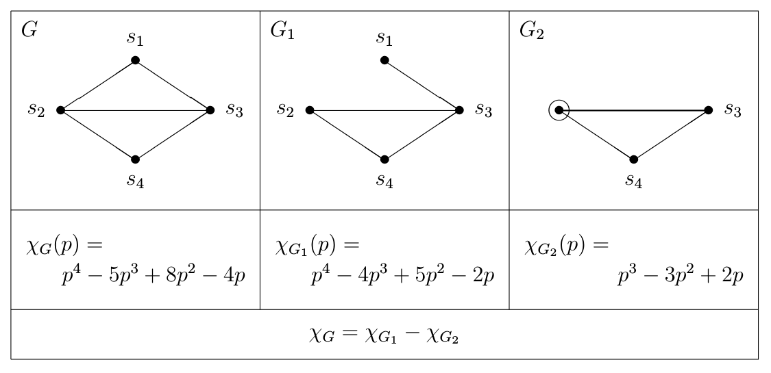
"We thus seek to deduce the chromatic polynomial of $G$ from chromatic polynomials of graphs *immediately simpler* than $G$. If the graph $G$ has no edges (in which case it is only a set of n unconnected vertices), then any coloring is a good coloring of $G$, so that $\\chi_G (p) = p^n$, and $\\chi_G$ is therefore already a polynomial. Otherwise the graph has at least one edge, for example, between the vertices $s_1$ and $s_2$. From graph $G$ two other graphs, $G_1$ and $G_2$, can be derived: The first, $G_1$, is obtained simply by deleting the edge between $s_1$ and $s_2$. The second, $G_2$, is obtained by *contracting* that same edge and convert its two ends into a single vertex of the graph $G_2$. We note that if $s_1$ and $s_2$ both were connected by edges to the vertex $s_k$, then the *two* old edges would be replaced by only *one* edge in the new graph.\n",
"\n",
"\n",
"\n",
"Consider a good coloring of $G_1$. If the two vertices $s_1$ and $s_2$ have the same color, a good coloring of $G_2$ is derived by \"collapsing\", however, the corresponding coloring of $G$ is not good. Conversely, if $s_1$ and $s_2$ have different color, a good coloring of $G$ can be derived, but it is no longer possible to derive a coloring of $G_2$ therefrom. It is easy to see that any good coloring of $G$ and $G_2$ could be obtained in this way. If $p$ is the number of colors, it follows immediately that $\\chi_G (p) = \\chi_{G_1} (p) - \\chi_{G_2} (p)$ or, if this is true for any integer $p$, $\\chi_G = \\chi_{G_1} - \\chi_{G_2}$, which is a relationship between polynomials, and the desired recurrence relation is maintained. We already deduce, by induction, that the chromatic polynomial... is indeed a polynomial! Once this is understood, it is a child's play to derive a recursive program for calculating $\\chi_G$ given $G$. The chromatic number of $G$ can then be obtained as a by-product. This last program, which is based on a simple recurrence, is considerably better than the one described previously.\n",
"\n",
"But it may be time to return to our subject, *infinity and effectiveness*. What is the relationship with our graph problem? It has been emphasized that the *chromatic polynomial* information is much richer than the *chromatic number* information: in a certain way it contains an *infinity* of information since this polynomial is defined *for any* number of colors $p$. Of course, this *infinity* of information cannot be described as such. The *functional trick* is used. Rather than considering the *set* of all pairs $(p,\\chi_G(p))$, we prefer to consider the *function* $\\chi_G$. For a bourbakist mathematician there is no difference since he defines a function as a set of argument-value pairs! But for a computer scientist it is quite different, because she can code this *infinity* of couples as a *polynomial* and thus in the form of a finite sequence of coefficients and exponents, which *can be stored in a machine*! This polynomial can be considered as a *program*, a finite text, *capable*, if asked, of giving a response, a value, whatever integer (here a number of colors) is communicated to it. This general scheme only works well because one is able to write and use programs that admit polynomials (programs) as input and provide as output another polynomial (program). This is necessary when using the recurrence formula. This kind of work is easy for polynomials but a little more difficult for algorithms of a a more general nature which will be examined later.\n",
"\n",
"If this phenomenon and its solution have been described so carefully, it is because they are closely related to what will be described in the last section of this paper about a very active but more esoteric field of research, that of *algebraic topology*: The two problems (and their solutions) are indeed of identical natures.\n",
"\n",
"# The lambda calculus.\n",
"\n",
"In the world of lambda-calculus there are only functions, as opposed to ordinary programming, where, in particular in courses for beginners (think of the perforated cards of yesteryear), the *program* (some text) is carefully distinguished from the *data* (another text, on which the program must work). In lambda-calculus there exist only functions which can serve interchangeably as programs or data. One mechanism, the *reduction* (described briefly in the article by M. Parigot), defines by what process the coupling of two functions, the first considered as a program, the second as data, sets in motion a theoretical machine which eventually produces a result (again a function) to be considered as the result of the program function working on the data function. It can also happen that the machine turns indefinitely in which case the result is indefinite.\n",
"\n",
"A lambda-calculus function is a text written in an entirely ordinary alphabet which consists of letters and some ad hoc signs, and obeys a few simple rules (a grammar). One can, if you like, consider such a text as a program written in the lambda-calculus language. This uniformity of nature, any object is a function, requires some acrobatics when dealing with ordinary data such as an integer. The lambda-calculus trick consists in coding an integer $n$ as the function that assigns to any function $f$ the function\n",
"\n",
"$$\n",
"\\underbrace{f\\circ f \\circ f\\circ\\ldots\\circ f}_{n}\n",
"$$\n",
"\n",
"It may seem overly complicated to encode an object as simple as an integer. Still, it is perfectly possible to program any recursive function in lambda-calculus. In section 2 of the article by M. Parigot, the realization of the addition of 2 and 2 in lambda-calculus is explained in great detail!\n",
"\n",
"The interest in lambda-calculus stems from the fact that, as a programming language, *programs capable of working on programs as input while producing programs as output* can be written in it.\n",
"\n",
"The story of lambda-calculus is rather curious. It was conceived and developed by the logicians of the 1930s to formalize the algorithmic aspect of mathematics in a sufficiently simple manner, and thus allowing to formulate a negative answer to Hilbert's conjecture regarding the existence of a universal algorithm capable of solving all mathematical problems. The proof is inspired by Gödel's incompleteness theorem and requires the admission of statements that can work on themselves. In terms of algorithms, it is necessary to consider programs capable of working on themselves. But this is obviously impossible if, in the programming environment, one carefully separates programs and data!\n",
"\n",
"Church's solution was to create an ingenious algorithmic model with only programs: this is the lambda-calculus.\n",
"Church thus contradicted Hilbert's conjecture. Turing reached the same conclusion by constructing instead an algorithmic model (Turing machine) where a program is nothing but data! Thus Turing discovered the very notion and the theoretical realization of a universal machine, which is the foundation of modern computer science. It can also be shown that Church's and Turing's solutions are equivalent.\n",
"\n",
"\n",
"# The manipulation of functional objects in a machine.\n",
"\n",
"The preceding sections can be summarized as follows: an apparently infinite object can sometimes be coded in the form of a finite text which represents a certain *function*. The example of the chromatic polynomial shows, however, that this *trick* is truly productive only if means are available to *calculate* other functional codings. Let us clarify this point!\n",
"\n",
"In the example of the chromatic polynomial we looked at functions whose domain and range are the set $\\mathbb{N}$ of the (non-negative) integers. As it turns out, these functions are in fact polynomials. This allows us to write - it would be better to say *encode* - them in the form of a finite text which consists of signs, coefficients, and of an insignificant letter (for example, $x$), and of exponents. By very simple conventions it is possible to represent such a polynomial, for example, as an ASCII string. The *chromatic polynomial* program must then be able to determine the *difference* polynomial of two given polynomials, in order to exploit the recurrence formula described earlier. More precisely, one must be able to write in the programming language used a two-argument function (the two *representations* of polynomials), which returns a representation of the difference polynomial. This is a simple exercise regardless of the programming language.\n",
"\n",
"It is easy because our functions are very special: they are polynomial functions. This exercise becomes much more difficult if one wants to handle functions of *any* kind. The first question is one of *coding*: How can one *encode*, in the form of a *finite* string, any function whose domain and range is the set $\\mathbb{N}$ of integers? The alphabet is finite, the set of these strings is enumerable, whereas, on the contrary, the set of functions $\\mathbb{N}\\rightarrow\\mathbb{N}$ has the cardinality of the continuum! Whatever the ingenuity of the writing system, it will only be possible to code a subset of all of these functions.\n",
"\n",
"Which functions should be selected? How should they be written? How can one write a program which relates, for example, the texts of two such functions to the text of the *difference* function? It turns that logicians, well before computer scientists and computer science, had given much thought to these questions. A good set of functions to select is the set of recursive functions, which, by a certain measure, is a very small subset of the set of all functions. But, in a certain sense, they are the only ones that are interesting! Various methods have been devised to represent them. They have all been demonstrated to be equivalent in terms of their capabilities.\n",
"\n",
"One of the most interesting representations is *lambda-calculus*. Luckily, the previous issue of Images de Mathématiques contained an excellent article by Michel Parigot entitled \"Proofs and programs: mathematics as\n",
"programming language,\" where he explained, among other things, lambda-calculus. See in particular the section *lambda-calculus as a machine language* and section 2 *normalization and lambda-calculus*. Readers who don't have time and energy to refer to Parigot's article might be satisfied with the indications given in section 4 of the present article.\n",
"\n",
"Unlike the Turing machine which ritually appears at the beginning of every theoretical computer course, the lambda-calculus was almost forgotten at the beginning of this half-century. It first reappeared in the research of the American computer scientist McCarthy who created the *Lisp* language at the end of the fifties of the last century. This programming language, which began out of simple curiosity and without the possibility of concrete applications worthy of the name, is in effect directly inspired by lambda-calculus. Like any formal mathematics, lambda-calculus rapidly produces *terms* whose length is such that it rules out any practical use: very quickly, this length exceeds for example the number of atoms of our galaxy! McCarthy reflected on methods (essentially the use of symbols as abbreviations) which would make it possible to overcome this difficulty. It was a long and difficult task. Sixty years later it is clear that in its current version, *Common Lisp*, it is one of the most powerful programming languages available! For example, the best formal computing systems such as Macsyma, Reduce, Scratchpad, etc, software of a very high complexity, are all based on Lisp.\n",
"\n",
"Since Lisp is directly inspired by lambda-calculus, it can easily, *during the execution of a program*, create programs which in turn are able to work on other programs to create others... This opens possibilities that are quite inaccessible to ordinary programming Pascal-style languages (Fortran, Ada, C, etc.). And these are precisely the capabilities that one needs to solve the problems of processing *functional code* objects that are considered here. \n",
"\n",
"For example, the Lisp function which, given two functions on $\\mathbb{Z}$ with values in $\\mathbb{Z}$, returns the difference function, is written quite simply:\n",
"```\n",
"(setf sub-functions\n",
" #'(lambda (f g)\n",
" #'(lambda (n) (- (funcall f n) (funcall g n)))))\n",
"```\n",
"The program text can be that reads as follows: The function `sub-functions` requires two arguments `f` and `g` (two functions) and maps them to the function which, given an integer `n`, assigns to it the difference of the two integers obtained by applying `f` and `g` to `n`. Here, we shall not attempt to explain the presence of the \"cabalistic\" signs `#` and `'`. They allow for certain optimizations and scope of identifiers, and are not available in ordinary languages, but we won't discuss them here.\n",
"\n",
"In the follwoing sequence of Lisp expressions\n",
"```\n",
"(setf f1 #'(lambda (x) (* x 3)))\n",
"(setf f2 #'(lambda (x) (* x x)))\n",
"(setf f3\n",
" (funcall sub-functions f1 f2))\n",
"```\n",
"the function $f_1 (x) = 3x$ and the function $f_2 (x) = x^2$ are defined, and then, *from the codes of these functions*, Lisp constructs the code of the difference function $f_3 = f_1 - f_2$.\n",
"\n",
"One can continue indefinitely in the same spirit and write, for example, a function whose argument is a binary operator on the integers. This function will return the function which is capable of working on pairs of functions $\\mathbb{N}\\rightarrow\\mathbb{N}$ according to the operator in question:\n",
"```\n",
"(setf create-op-function\n",
" #'(lambda (operator)\n",
" #'(lambda (f g)\n",
" #'(lambda (n)\n",
" (funcall operator (funcall f n) (funcall g n))))))\n",
"```\n",
"which one can read as: \"will provide the function which, with two functions $f$ and $g$, will associate the function which, to $n$, ...\". And instead of defining our function `sub-functions` as above, we could simply obtain the same result by:\n",
"```\n",
"(setf sub-functions (funcall create-op-function #'-))\n",
"```\n",
"\n",
"# Simplical complexes.\n",
"\n",
"It is hoped that the preceding section will have reassured the reader as to the possibilities of processing functional objects in a machine, even *during* program execution. In this section, we explain how it is possible to use the functional trick to encode *geometric* objects that can be quite monstrous. Playing with monsters in a machine is not, however, a goal in itself, and the few monsters exhibited in this section actually have no real interest. In the next section, we will explain how the same methods allow us to work on machines with highly infinite and *really useful* spaces (at least for mathematicians!). The example of loop spaces, which is easy to understand, is ideal to illustrate our purpose.\n",
"\n",
"Let us first explain what a *simplicial complex* is. The definition is *combinatorial*, but there is a *geometrical* object associated with any simplicial complex, the one we want to model by the combinatorial definition: a *simplicial complex* $K$ is a pair $K = (V, S)$ where $V$ is any set, the set of vertices of $K$, and $S$ is a set of *finite* subsets of $V$, the set of *simplices* of $K$. These data must satisfy the following conditions:\n",
"\n",
"1. If $v$ is a vertex of $K$, in other words, if $v\\in V$, then $\\{v\\}\\in S$;\n",
"2. If $s$ is a simplex of $K$, in other words, if $s\\in S$, and if $s'\\subset s$, then $s'\\in S$: any sub-simplex of $K$ is still a simplex of $K$.\n",
"\n",
"Let's say for example $K_1=(V_1,S_1)$, where\n",
"$$\n",
"\\begin{aligned}\n",
"V_1=\\big\\{ & 0,1,2,3,4,5 \\big\\}, \\mathrm{and}\\\\\n",
"S_1 = \\big\\{ & \\{\\}, \\\\\n",
" & \\{0\\},\\{1\\},\\{2\\},\\{3\\},\\{4\\},\\{5\\},\\\\\n",
" & \\{0,1\\},\\{0,2\\},\\{1,2\\},\\{2,3\\},\\{3,4\\},\\{3,5\\},\\{4,5\\},\\\\\n",
" & \\{0,1,2\\}\\big\\}.\n",
"\\end{aligned}\n",
"$$\n",
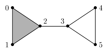
"The complex $K_1$ has six vertices and fifteen simplices. The associated the geometric object can represented as shown in the following figure:\n",
"\n",
"\n",
"\n",
"The triangle 012 is *filled* while the triangle 345 is *hollow*. The method of correspondence between lists of vertices and simplices on the one hand and geometric objects on the other hand is clear: the figure associated with a simplicial complex has as many \"marked points\" as there are vertices in the complex. Two marked points are connected by a segment if the set of these two vertices is included in the list of simplices. Three vertices underlie a full triangle, if all of all three vertices appear in the list of simplices, etc. It can be shown that, by chosing a Euclidian space of a sufficiently high dimension, one can always associate with a simplicial complex, sometimes called an *abstract* simplicial complex, a geometrical object of this nature, which is then called a *geometric* simplicial complex.\n",
"\n",
"Here's another example. With the abstract simplicial complex:\n",
"\n",
"$K_2=(V_2,S_2)$, where\n",
"$$\n",
"\\begin{aligned}\n",
"V_2=\\big\\{ & 0,1,2,3\\big\\}, \\mathrm{and} \\\\\n",
"S_2 = \\big\\{ & \\{\\}, \\\\\n",
" & \\{0\\},\\{1\\},\\{2\\},\\{3\\},\\\\\n",
" & \\{0,1\\},\\{0,2\\},\\{0,3\\},\\{1,2\\},\\{1,3\\},\\{2,3\\},\\\\\n",
" & \\{0,1,2\\}, \\{0,1,3\\}, \\{0,2,3\\}, \\{1,2,3\\}\\big\\}.\n",
"\\end{aligned}\n",
"$$\n",
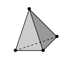
"we can associate the hollow tetrahedron:\n",
"\n",
"\n",
"\n",
"It is hollow because in the list of its simplices the simplex $\\{0,1,2,3\\}$ *does not appear*. Otherwise the associated geometrical object would have been a *solid* tetrahedron.\n",
"\n",
"A *finite* simplicial complex can easily be machine-coded as a list of simplices. In fact, one could be content with the maximal simplices, the others being deducible. Thus our first example of a simplicial complex could be coded:\n",
"```\n",
"((0 1 2) (2 3) (3 4) (3 5) (4 5))\n",
"```\n",
"While the hollow tetrahedron would be written:\n",
"```\n",
"((0 1 2) (0 1 3) (0 2 3) (1 2 3))\n",
"```\n",
"And the solid tetrahedron:\n",
"```\n",
"((0 1 2 3))\n",
"```\n",
"\n",
"Nothing prevents us from considering *infinite* simplicial complexes. Consider, for example, the complex $K_3 = (V_3, S_3)$ where $V_3$ is the set of natural numbers and $S_3$ the set of all finite subsets of $\\mathbb{N}$.\n",
"\n",
"$K_3=(V_3,S_3)$, where\n",
"$$\n",
"\\begin{aligned}\n",
"V_3=\\big\\{ & 0,1,2,3,4,5,6,7,8,\\ldots\\big\\}, \\mathrm{and}\\\\\n",
"S_3 = \\big\\{ & \\{\\}, \\\\\n",
" & \\{0\\},\\{1\\},\\{2\\},\\{3\\},\\{4\\},\\{5\\},\\{6\\},\\{7\\},\\ldots\\\\\n",
" & \\{0,1\\},\\{0,2\\},\\{0,3\\},\\{0,4\\},\\{0,5\\},\\{0,6\\},\\ldots\\\\\n",
" & \\{1,2\\},\\{1,3\\},\\{1,4\\},\\{1,5\\},\\{1,6\\},\\ldots\\\\\n",
" & \\{2,3\\},\\{2,4\\},\\{2,5\\},\\{2,6\\},\\ldots\\\\\n",
" & \\ldots\\\\\n",
" & \\{0,1,2\\}, \\{0,1,3\\}, \\{0,1,4\\}, \\{0,1,5\\},\\ldots\\\\\n",
" & \\{0,2,3\\}, \\ldots\\\\\n",
" & \\ldots \\\\\n",
" & \\{0,1,2,3\\},\\ldots\\\\\n",
" & \\ldots\\\\\n",
" & \\ldots\\big\\}.\n",
"\\end{aligned}\n",
"$$\n",
"\n",
"The associated geometric object contains a segment for any pair of different integers, a solid triangle for any triplet of pairwise different integers, a solid tetrahedron for any quadruplet of pairwise different integers, and so on. Obviously, such an object cannot be represented in $\\mathbb{R}^3$, but it is not difficult to define rigorously a geometrical object in $\\mathbb{R}^\\infty$ corresponding to the simplicial complex $K_3$. Here's another example, which is somewhat of a *sub-example* of the preceding one: Take $K_4 = (V_4, S_4)$ where $V_4$ is still the set $\\mathbb{N}$ of natural numbers, and $S_4$ is the set of subsets of $\\mathbb{N}$ which contain *at most* two elements:\n",
"\n",
"$K_4=(V_4,S_4)$, where\n",
"$$\n",
"\\begin{aligned}\n",
"V_4=\\big\\{ & 0,1,2,3,4,5,6,7,8,\\ldots\\big\\}, \\mathrm{and}\\\\\n",
"S_4 = \\big\\{ & \\{\\}, \\\\\n",
" & \\{0\\},\\{1\\},\\{2\\},\\{3\\},\\{4\\},\\{5\\},\\{6\\},\\{7\\},\\ldots\\\\\n",
" & \\{0,1\\},\\{0,2\\},\\{0,3\\},\\{0,4\\},\\{0,5\\},\\{0,6\\},\\ldots\\\\\n",
" & \\{1,2\\},\\{1,3\\},\\{1,4\\},\\{1,5\\},\\{1,6\\},\\ldots\\\\\n",
" & \\{2,3\\},\\{2,4\\},\\{2,5\\},\\{2,6\\},\\ldots\\\\\n",
" & \\ldots\\\\\n",
" & \\ldots\\big\\}.\n",
"\\end{aligned}\n",
"$$\n",
"\n",
"This time the associated geometrical object will contain an infinity of segments, but on the other hand no triangle, no tetrahedron, ...\n",
"\n",
"Of course, it is absolutely impossible to represent such simplicial complexes using lists of simplices. Only lists of finite length can be represented in a machine, and the lists which would be needed for the complexes $K_3$ and $K_4$ are infinite. Given the preparations of the previous sections, the reader will probably guess that we will use the *functional trick* to overcome this difficulty. How should we proceed?\n",
"\n",
"We may decide the functional coding for a simplicial complex is a function $f$ which can be applied to any list of machine objects and which returns **true** or **false**. In addition, this function must satisfy the following condition: if $f(l) = \\mathbf{true}$ and $l'\\subset l$, then $f(l')=\\mathbf{true}$. It is easy to associate a simplicial complex with such a function $f$: let $V_f$ be the set of objects $v$ such that $f\\big(\\{v\\}\\big) = \\mathbf{true}$, and $S_f$ the set of all lists for which $f$ answers $\\mathrm{true}$. Then $K_f = (V_f, S_f)$ is a simplicial complex called the simplicial complex associated with $f$. By this very simple process, the simplicial complexes are *functionally* coded. Since the function $f$ can *potentially* work on an infinite number of objects (see section 2), nothing prevents us from coding infinite simplicial complexes.\n",
"\n",
"The various examples of complexes which have been given previously can be coded in Lisp as follows:\n",
"\n",
"```\n",
"(setf K1\n",
" #'(lambda (list)\n",
" (or (subsetp list '(0 1 2))\n",
" (subsetp list '(2 3))\n",
" (subsetp list '(3 4))\n",
" (subsetp list '(4 5))\n",
" (subsetp list '(3 5)))))\n",
"```\n",
"\n",
"If we interrogate `K1` for the list `(0 2)`, it will answer **true**, whereas it will answer **false** for example for the list `(0 3)`. The hollow tetrahedron might be coded like this:\n",
"\n",
"```\n",
"(setf K2\n",
" #'(lambda (list)\n",
" (and (subsetp list '(0 1 2 3))\n",
" (not (subsetp '(0 1 2 3) list)))))\n",
"```\n",
"\n",
"This requires that all elements of the argument list can be extracted from the list `(0 1 2 3)`, but all elements of the latter list must not appear at the same time. If this last condition were removed, one would have the functional code of the full tetrahedron. The functional code of the infinite complex $K_3$ is not much longer. It is even shorter:\n",
"\n",
"```\n",
"(setf K3\n",
" #'(lambda (list)\n",
" (every #'integerp list)))\n",
"```\n",
"\n",
"It is enough to check that every element of the list argument is an integer, which, as we see, can easily be written. \n",
"\n",
"Let $K_4$ be the complex $K_3$ with all the simplices of dimension $> 1$ removed. Topologists call $K_4$ the 1-skeleton of $K_3$, and it can be functionally coded as follows:\n",
"```\n",
"(setf K4\n",
" #'(lambda (list)\n",
" (and (every #'integerp list)\n",
" (< (length (remove-duplicates list))\n",
" 3))))\n",
"```\n",
"\n",
"Indeed, this time it is necessary to verify additionally that the number of *different* vertices in the list is less than 2.\n",
"\n",
"This description of $K_4$ as the 1-skeleton of $K_3$ is a good opportunity to illustrate some of the functional possibilities of Lisp: we would like to have a function to which we pass two arguments, where the first argument is the functional code of a simplicial complex $K$, and the second argument is a dimension $d$. We want this function to *produce* a functional code of the $d$-skeleton of $K$, which is the new simplicial complex obtained from $K$ by *removing* all the simplices of dimension $>d$. This is very easy:\n",
"\n",
"```\n",
"(setf skeleton\n",
" #'(lambda (complex dimension)\n",
" #'(lambda (list)\n",
" (and (funcall complex list)\n",
" (< (length (remove-duplicates list))\n",
" (+ 2 dimension)))))\n",
"```\n",
"\n",
"So that instead of getting tired from writing a functional code of $K_4$, one could have asked the Lisp machine to do it:\n",
"\n",
"```\n",
"(setf K4 (funcall skeleton K3 1))\n",
"```\n",
"\n",
"\n",
"# Constructing a loop space in a machine.\n",
"\n",
"Let $K = (V,S)$ be a simplicial complex and $s_0$ one of its vertices, which will play a particular role and which is called the *base point* of $K$. We assume that $K$ is *connected*, in other words, starting from the base point, any other vertex is *accessible* by traveling along the edges of $K$. The loop space of $(K, s_0)$, which we denote by $\\Omega(K,s_0)$, is another simplicial complex defined from $K$ and $s_0$, which is always infinite (except when $V = \\{s_0\\}$). This loop space plays a particularly important role in algebraic topology: it was invented by Jean-Pierre Serre in the early fifties and in a certain sense acts as the *inverse space* of $K$. This is not the place to define in what sense, but it is the type of construction that allowed Jean-Pierre Serre to advance the \"state of the art\" in Algebraic Topology (the homotopy groups of the spheres), a contribution which earned him the Fields Medal.\n",
"\n",
"It is not difficult to define the loop space and it gives a striking example of the possibilities offered by *functional coding* methods. Since $K = (V, S)$ is given, as well as a vertex $s_0$ of $V$, the *complex* $\\Omega(K, s_0)$, *the loop space of* $(K, s_0)$ is, like every complex, defined by its set of Vertices $V'$ and its set of simplices $S': \\Omega(K, s_0) = (V',S')$.\n",
"\n",
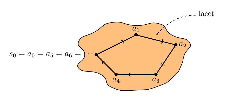
"Let us first describe the set of vertices $V'$. A vertex of $\\Omega(K, s_0)$ is a loop of $K$ based on $s_0$, by which we mean an infinite sequence of vertices $(a_0, a_1, a_2,\\ldots, a_{k-1}, a_k,\\ldots)$ satisfying the following conditions:\n",
"\n",
"a) The first vertex of this sequence must be the base point $s_0$ of $K$: $a_0 = s_0$;\n",
"\n",
"b) There must be an integer $n$ such that, if $k \\geq n$, then $a_k = s_0$;\n",
"\n",
"c) For every integer $k > 0$, $\\{a_{k-1},a_k\\}$ is a simplex of $K$: $\\{a_{k-1},a_k\\}\\in S$ (repetition is permitted, in which case this simplex has only one element).\n",
"\n",
"\n",
"\n",
"This sequence must be understood as a *path* on $K$, more precisely along the edges of $K$. At time 0, we start from the base point: $a_0 = s_0$; at time 1, one reaches the vertex $a_1$ of $K$, which, to be legitimate, requires that $\\{a_0,a_1\\}$ be a simplex of $K$. Intuitively, between times 0 and 1, the loop runs *along* the edge of $K$ between $a_0$ and $a_1$. Similarly, between the instants $k-1$ and $k$, the loop runs along the edge of $K$ between $a_{k-1}$ and $a_k$, which requires that $\\{a_{k-1},a_k\\}$ belongs to $S$. We also require that this journey be essentially finite, which is the role of condition b): after a certain time $n$, the loop remains fixed at the base point $s_0$ of $K$. For example, if $K$ is the example complex $K_1$ of the preceding section with the base $s_0 = 2$, the following sequence $\\lambda = (2, 3, 4, 5, 3, 4, 5, 3, 2, 2, 2,\\ldots)$ is an example of a *vertex* of $\\Omega(K_1, 2)$.\n",
"\n",
"Thus the data of a *single* vertex of $\\Omega(K, s_0)$ requires several vertices and edges of $K$. Let us now define the simplices of $\\Omega(K, s_0)$. For example, let $\\lambda=(a_0,a_1,\\ldots)$ and $\\lambda'=(a'_0,a'_1,\\ldots$ be two vertices of $\\Omega(K, s_0)$. Under what circumstances is the pair $\\{\\lambda,\\lambda'\\}$ a simplex of $\\Omega(K, s_0)$? The condition that must be satisfied is the following:\n",
"\n",
"> For each integer $k > 0$, the set $\\{a_{k-1},a_k,a'_{k-1},a'_k\\}$ (repetitions are allowed) must be a simplex of $K$: $\\{a_{k-1},a_k,a'_{k-1},a'_k\\}\\in S$.\n",
"\n",
"The interpretation of this condition is not difficult. It requires that one be able to define an *intermediate* path between the paths $\\lambda=(a_0,a_1,\\ldots)$ and $\\lambda'=(a'_0,a'_1,\\ldots)$. At the instant $k \\in \\mathbb{N}$, this intermediate path should pass through the middle of the segment $[a_k,a'_k]$, which requires to be defined that $\\{a_k,a'_k\\}$ belongs to $S$.\n",
"\n",
"Better, at instant $k-\\frac{1}{2}$, the intermediate path must pass through the middle of the segment $\\big[\\lambda(k-\\frac{1}{2}),\\lambda'(k-\\frac{1}{2})\\big]$, which is also the barycenter of the four points $\\lambda(k-1), \\lambda(k),\\lambda'(k-1)$ and $\\lambda(k)$, in other words, $a_{k-1},a_k,a'_{k-1}$ and $a'_k$. Therefore, for this barycentre to be defined, we ask that these four points define a simplex of the complex $K$ (repetitions are permitted). For example, for the example complex $K_1$ of the previous section, if we take $\\lambda=(2,3,4,5,3,2,2,2,\\ldots)$ and $\\lambda'=(2,3,3,4,5,3,2,2,...)$, this condition is not satisfied at time 3 since $\\{3,4,5\\}$ does not belong to $S$, and so $\\{\\lambda,\\lambda'\\}$ *is not* a simplex of $\\Omega(K_1,2)$. On the other hand, if we take $\\mu=(2,0,1,2,2,2,\\ldots)$ and $\\mu'=(2,2,0,1,2,2,\\ldots)$, the condition is always satisfied, essentially because $\\{0,1,2\\}$ belongs to $S$, and therefore $\\{\\mu,\\mu'\\}$ is an element of $S'$: $\\{\\mu,\\mu'\\}$ *is* a simplex of $\\Omega(K_1,2)$.\n",
"\n",
"More generally and in the same spirit, let $\\lambda^i=(a_0^i,a_1^i,a_2^i,\\ldots), 1\\leq i\\leq m$, be a family of loops of $\\Omega(K, s_0)$. This family will constitute a simplex of $\\Omega(K, s_0)$ if and only if, for every integer $k > 1$, the family $\\{a_{k-1}^1,a_k^1,a_{k-1}^2,a_k^2,\\ldots,a_{k-1}^m,a_k^m\\}$ belongs to $S$, which, intuitively, makes it possible to define a *barycentre* path of the paths $\\lambda^1,\\ldots,\\lambda^m$.\n",
"\n",
"Let us now examine the possibility of constructing a function with two arguments where the first argument is the functional code of a simplicial complex and the second argument is one of its vertices (the base point), and which returns the functional code of its loop space. This last code must be able to work on lists and must answer 'yes' or 'no' to the question: *is this list a simplex of the loop space complex*? Each list element must be a vertex, which poses a bit of a problem, because a vertex of the loop space has been defined as an *infinite* sequence. But this problem is easy to overcome since condition b) ensures that, starting from a certain rank, which might vary from one sequence to another, all the terms of this sequence are equal to the base point. It is therefore sufficient that such a sequence is represented in the form of a *finite* list, where all the missing terms are equal to the base point. The test of the conditions to be satisfied in order for a list of lists to represent (modulo this convention) a simplex of our loop space is then a small program using inter alia the *functional code of the original complex*. The program transformation of the functional code of a complex to the functional code of its loop space can itself be implemented, for example, by the following program which is shown only to satisfy the possible curiosity of the reader:\n",
"```\n",
"(setf loop-space\n",
" #'(lambda (K s0)\n",
" #'(lambda (ll)\n",
" (and (maplistp ll)\n",
" (let ((ll (transpose (complete ll s0))))\n",
" (essential-test K ll)))))\n",
"```\n",
"The `loop-space` function uses various auxiliary list-processing functions (`maplistp`, `transpose`, `complete`, `essential-test`) whose implementation is a routine programming exercise. As a result, a very modest microcomputer *calculates* in less than one hundredth of a second the functional code of a loop space, a space yet highly infinite!\n",
"\n",
"\n",
"# Applications to algebraic topology.\n",
"\n",
"In this last section, we describe very briefly the results that can be obtained from this method of functional coding when applied to algebraic topology. The situation is very similar to that which has been explained for the chromatic polynomial and the parallelism is summarized in Table 1.\n",
"\n",
"The object of the algebraic topology is to associate with (topological) spaces algebraic objects capable of essentially measuring some of their properties. The *homology groups* are a very important example of such an association, however, their precise definition is too esoteric to be explained here. In a way, these groups measure how *perforated* a space is. For example, topologists explain that the first homology group of the Euclidean plane $\\mathbb{R}^2$, denoted by $H_1(\\mathbb{R}^2)$, is zero, whereas if $D$ is the unit disk of this plane, $H_1(\\mathbb{R}^2-D)$ is not zero, which expresses the fact that $\\mathbb{R}^2-D$ is *punctured*. In the present case, this can be seen on the group $H_1$ since the hole in question can be enclosed in a circle, an object of dimension 1. If we did the same for the Euclidean space $\\mathbb{R}^3$ and its unit ball $B$, it would be this time the group $H_2$ which would be non-zero, because the corresponding hole can be enclosed in a sphere, a two-dimensional object. Algebraic topologists can define very precisely these notions which produce, for a space $K$, the homology groups $H_n(K)$, for every positive integer $n$.\n",
"\n",
"The calculation of the homology groups of many spaces of interest to topologists is a difficult sport and remains a very active research topic today. It is this type of calculation where functional coding methods have recently made significant progress, very much as the chromatic polynomial method makes it possible to simplify the calculation of the chromatic number. The parallel between the two situations is fairly well summarized in this table:\n",
"\n",
"| Graphs | Algebraic Topology |\n",
"|--------|--------------------|\n",
"| Graph $G$ | Simplicial set $K$ |\n",
"| Chromatic number | Ordinary homology |\n",
"| Known chromatic number $N_G$
Simple construction of $G'$ from $G$
$N_{G'}=???$ | Known ordinary homology $H_*(K)$
Simple construction of $K'$ from $K$
$H_*(K')=???$ |\n",
"| Chromatic polynomial $\\chi_G$ | Effective homology $EH_*(K)$ |\n",
"| The chromatic polynomial contains an infinity of information | The effective homology contains an infinity of information |\n",
"| *Functionally* coded information; on a machine, this information appears as a *finite* string of bits | *Functionally* coded information; on a machine, this information appears as a *finite* string of bits |\n",
"| The chromatic polynomial contains the chromatic number as a *by-product* | The effective homology contains the ordinary homology as a *by-product* |\n",
"| Construction of $G$ from $G_1, G_2$
Algorithm for $N$ from $N_1,N_2$ | Construction of $K$ from $K_1, K_2$
Algorithm for $EH$ from $EH_1,EH_2$\n",
"\n",
"There is, however, a slight difference in the case of algebraic topology: many methods (exact sequences and spectral sequences in particular) had already been developed by topologists, so that when we construct a space $K$ from spaces $K_1$ and $K_2$ whose homologies are known, we can glean at least some information about the homology of $K$. Often we can even deduce the homology of $K$, but often these methods prove insufficient.\n",
"\n",
"The methods of *effective homology*, developed by the author in collaboration with other researchers (see references at the end of the article), make it possible to overcome the difficulties presented by the other methods. The constraints of this article do not allow much more explanation. Let us say only that the objects with *effective homology* contain, like a chromatic polynomial, an infinity of information, but the *functional trick* nevertheless allows to manipulate them without any particular difficulty on theoretical and concrete machines. The classical methods of algebraic topology are thus transformed into true *algorithms* that are capable of computing the coveted groups.\n",
"\n",
"Numerous computability results have already been obtained in this way, in particular for the homology groups of iterated loop spaces. By implementing these methods on concrete machines, it would be most interesting of course to calculate the homology and homotopy groups that have hitherto resisted such attempts. A lot of work is going on in this direction, specifically for the homology of iterated loop spaces.\n",
"\n",
"The wide field of research, which ranges from the purest mathematics (homological algebra and algebraic topology) to the very concrete problems of the realization of algorithms on machines, is exciting. It also opens unexpected horizons for researchers in complexity (what can we say about the complexity of algorithms based on functional programming?) and parallel computation.\n",
"\n",
"\n",
"**To learn more:**\n",
"\n",
"- Francis SERGERAERT. *Homologie effective*, I et II. C. R. Acad Sc. Paris, Série I, 1987, vol. 304, pp 279-282 et 319-321.\n",
"- Julio RUBIO, Francis SERGERAERT. *Homologie effective et suites spectrales d'Eilenberg-Moore*. C. R. Acad. Sc. Paris, Série I, 1988, vol. 306, pp 723-726.\n",
"- Francis SERGERAERT. *The computability problem in algebraic topology*. Prépublication de l'Institut Fourier, n o 119, 1988.\n",
"- Julio RUBIO. *Homologie effective des espaces de lacets itérés*. Prépublication de l'Institut Fourier, no. 138, 1989"
]
}
],
"metadata": {
"kernelspec": {
"display_name": "SBCL Lisp",
"language": "lisp",
"name": "lisp"
},
"language_info": {
"codemirror_mode": "text/x-common-lisp",
"mimetype": "text/x-common-lisp",
"name": "common-lisp",
"pygments_lexer": "common-lisp",
"version": "X3J13"
}
},
"nbformat": 4,
"nbformat_minor": 2
}