
209 KiB
Common Lisp, Typing, and Mathematics
By Francis Sergeraert, August 2001
(Adapted for cl-jupyter by Gerd Heber, February 2017)
Introduction.
Common Lisp is seldom used by mathematicians and this is an anomaly. The high level of quality of Common Lisp comes from a simple reason: Common Lisp is a mathematical object, certainly one of the most beautiful and potentially productive existing at this time. Common Lisp is a descendant of the fantastic $\lambda$-calculus, designed by Church to produce one of the deepest mathematical results of the last century, namely the negative answer to Hilbert's Entscheidungsproblem ("decision problem"): no algorithm can determine whether an arbitrary mathematical statement is true, false or undecidable.
Then, by a quite indirect route, $\lambda$-calculus became a fascinating programming language, Lisp. Lisp's birth is old, at the end of the fifties, and forty years later it is clear it remains the most advanced "common" programming language, "common" meaning with an ANSI norm, in this case the $\ldots$ Common Lisp norm. The Common Lisp language is so advanced that it is not so easy to use it for serious applications: a reasonable lucidity about its complex and far-reaching structure is required; so that the initiation stage in the learning process of this language is a little hard. The present paper is a tutorial to introduce mathematicians to the main components of Object Oriented Programming in Common Lisp. The extraordinary work of Guy Steele and his X3J13 committee during the years 1980-1994 led to a powerful language, on one hand, but on the other hand taking seriously account of standard practical constraints in actual programming work. Common Lisp is now widely used for complex industrial applications, mainly because of the powerful dynamic tools that are available; but it is not used very much for scientific applications, in particular for mathematical applications, and this must be corrected.
No concrete language can be completely formalized, but the mathematical precision of the definition of Common Lisp gives its user much security, the precision which is required for sophisticated mathematical applications, in particular when complicated data-sharing arrangements are necessary. Another aspect of Common Lisp is without any equivalent with the other languages: the user may freely design his application at the best programming level, sometimes at a very high level, directly handling rich and complex mathematical structures; for example it is explained in Section 5.2 that three simple lines of Lisp code are sufficient to explain to the machine that a simplicial group is simultaneously a Kan space and a Hopf algebra, sharing a common graded differential coalgebra structure, but with some added data, namely two simplicial morphisms describing the simplicial group structure. Other times, in the same program, you may on the contrary work at a very low level, in an assembler-like style. The language is carefully stratified to help the developer to remain lucid and at ease about these questions. The Common Lisp macro generator, without any equivalent in other common languages, allows also the programmer to easily use his low level code when he is on the contrary working at a high level.
Which is a good element for appreciation is the ability of a language to be quickly adapted to new mandatory evolutions; at this time, Object Oriented Programming (OOP) must be integrated in a language claimed common, and Common Lisp succeeded in doing it so nicely that it can even be used to describe what OOP exactly is. The CLOS (Common Lisp Object System) chapter of [STEL2] is one of the most amazing parts of Computer Science. The general dynamic feature of Common Lisp has in particular been kept: the user may dynamically change the class of his objects; he may also redefine dynamically the classes without loosing the objects of this class; and the user may freely decide exactly what happens for these objects. If this is not yet flexible enough, the Metaobject Protocol (MOP), not yet ormalized, but already widely used, allows our user to freely define his own OP system; CLOS is in fact only a particular application of MOP, see [KCRB].
This paper is devoted to a few didactical examples to help mathematicians to understand how Common Lisp and more precisely CLOS can be used for mathematical applications. It is organized as follows. Firstly, a small set of artificial examples is used to explain the general structure of CLOS. The main work in OOP, and certainly the most difficult one, is at the initialization stage of the instances (objects). Even if a user does not intend to use the current Common-Lisp, studying how the initialization process is designed in this environment will explain to him the good points of view in this domain.
Then a more significant example is described to show the actual workstyle when CLOS is used in a non-beginner job. Because the OOP subject is strongly related to typing, a possible description of what typing could be is used as a theme of an exercise showing how CLOS allows to implement the consequences of this description. This example is very simple and should be a good tutorial to simultaneously understand the initial points of OOP under Common Lisp and what typing is, at least from the point of view of the actual programmer.
The next section is more mathematically oriented: it is explained how the basic mathematical categories, sets, magmas and monoids, can be directly implemented in CLOS, without meeting any kind of difficulty. The possibility for the Lisp user to arbitrarily mix OOP and high level functional programming (lexical closures) gives at once the required tools. The specialized programming environments such as Axiom, Gap, Magma $\ldots$ so can be skipped and the mathematician may freely work at an arbitrary level in the programming language itself, keeping a perfect control of the environment, without being bothered by a restrictive environment, seldom well-adjusted to an arbitrary new research work.
It was the case of the author and his colleagues when the central problems of Algebraic Topology were considered from a computational point of view [SRGR3][RBSR6]. The resulting Lisp program Kenzo [DRSS] shows a concrete example of use of CLOS for a relatively large implementation work1. The Kenzo program is not at all didactic, it is an actual program able to produce mathematical results that are unreachable otherwise. Some points of the experience acquired by Kenzo's authors are discussed in the last section and in this way the reader will see a few more concrete points of CLOS.
1 16000 Common Lisp lines and a 340pp documentation.
CLOS (= Common Lisp Object System).
Strictly speaking, the notion of Common Lisp Object System, CLOS in short, does not make sense anymore. The first definition of Common Lisp, known as Common-Lisp-1984 [STEL1], did not have any "object system". Typing was already strong in CL-1984, at least if wished by the user; standard types were defined and the initial type system was freely extendable by the user, but the now classical notions of classes, instances, generic functions and methods were not yet available. The pre-ANSI version of Common Lisp, namely Common-Lisp-1990, contained a proposal for an OOP system, called Common Lisp Object System Ch. 28, pp 770-864 [STEL2]; the pre-versions of this object system were already widely used at this time by the Lisp programmers. Finally, the ANSI specification [ANSI] of Common Lisp (1994) completely integrated the so-called Common Lisp Object System in the very definition of the language. The standard Lisp programmer is now assumed working according to the spirit of OOP, constantly using classes, instances of classes, methods and so on, like in C++ or Java2. But the perfect integration of the general ideas of OOP with the so powerful Common Lisp gives its user many capabilities which are at this time outside of scope with other languages, mainly when functional programming is involved. However we continue to call CLOS the part of the ANSI Common Lisp language devoted to OOP.
This object system in Common Lisp coexists with the old typing system and also the old structure system, which allowed the user to define, construct and use the classical record objects, with several fields, typed or not. From a hierarchical point of view, the typing system and the structure system are subsystems of the object system: special predefined classes correspond to the main classical data types, and the same for the structured objects. But normaly the current Lisp programmer mainly works with the object system, organizing his workspace in classes, subclasses, methods and so on.
The Common Lisp object system is elegant and powerful. As usual in Common Lisp, it is organized so that the user keeps a very large freedom. A standard style is carefully designed, but the user may go far from this standard style if special situations are encountered.
2 With a slightly different terminology.
A quick comparison with C++ and Java.
A few indications are given in this section about the main OOP features of Java, C++ and CLOS. In Java, the classes are "above" the methods (member functions): the specific functions for a class are defined inside this class so that the class and member function hierarchies are more or less parallel. This leads sometimes to artificial classes, typically the System class and the Math class, when this rule becomes non-sense in particular situations. The member functions are available under C++ too.
In C++ you may also overload the functions, in particular the member functions. There are no member functions in CLOS3, there is only an overloading feature. But three other features are provided by CLOS which make particularly convenient and elegant the developer work:
- The initialization process of the objects is essential in OOP; the general CLOS organisation of this work is really wonderful, in particular conceptually very simple, leading the programmer towards the good points of view, see Section 2.3 for a small introduction to this point.
- The method qualifiers give much flexibility to organize the work of all the applicable methods; numerous simple examples in this paper.
- The functional basis of Common Lisp allows the user to easily install functional slots (members) of any sort, in particular compiled closure slots, dramatically extending the programming scope; Section 4 gives striking applications of this feature; in particular the instances may be themselves funcallable, in other words the instances become also functional objects, see Section 3 for a typical illustration.
In CLOS, the basic ingredients are clearly distinguished:
- The class system, mainly used through the
defclassstatement, allows the user to define the structure of his instances (objects), in particular through the notion of subclass (derived class). - The function type is primitive; a function is an object which can be funcalled (called) for some work about some arguments.
- The packaging system allows the developer to precisely define what parts of his source code are normally directly known and/or reachable by a user of his program, obtaining in particular the equivalent of the
privateC++ code.
Then, if the class system and the functional organization of Common Lisp are to be simultaneously considered, the particular notions of generic functions and methods must be used.
- A generic function is a functional object the exact work of which will depend on the class of its arguments.
- The code for some specific work of a generic function corresponding to some particular class distribution of its arguments and some qualifier is a method object; each method is defined by a
defmethodstatement. - In general several methods are involved when a generic function is invoked, they are called the applicable methods. CLOS gives its user a large freedom to organize these methods with respect to each other, to cover any possible situation, in particular when a sophisticated chronology of their work is required. This feature has no equivalent in C++ or Java, this is obtained by the method qualifiers.
In this way, the CLOS methods can be thought of arranged in a three-dimensional array where each entry is associated to a generic function, the first index, the class distribution of the parameters, the second index, and the method qualifier, the third index.
The CLOS method qualifiers have no equivalent in C++ or Java; a predefined qualifier organization is provided, already rather rich, sufficient for most of the ordinary cases4. If still more sophisticated combinations of methods are required, the define-method-combination function allows the developer to freely extend this organization.
For example, and this will be detailed in Section 4, a mathematician who installs under CLOS the traditional mathematical categories must organize his work as follows:
- The
defclassstatements will be used to define what a set object is, what a group object is, what a chain complex object is, and so on. - The
defgenericstatements will be used to define functions working on these objects, but these "functions" are traditionnally called in this case functors in mathematics; therefore onedefgenericstatement for the sum functor, another defgeneric for the product functor, anotherdefgenericfor the classifying space functor, and so on. - Finally each generic function will have various methods to adapt the generic function to specific cases; for example the product of two objects of some category is also an object of this category with the corresponding structure to be defined. Therefore one product method for the sets, another product method for the magmas, another product method for the monoids, and so on. The
call-next-methodandchange-classfunctions will allow these methods to possibly refer to the less specific ones.
3 A C++ or Java member function is nothing but a CLOS generic function where the first argument is given before the function reference, with an implicit with-slots for this particular argument; such a feature can be easily added to the environment with the Metaobject Protocol; in general CLOS prefers to keep the maximal symmetry between the critical arguments.
4 For example quite sufficient for the Kenzo program.
Very simple CLOS examples.
Classes can be defined with the traditional hierarchy and methods may be defined which will be called, or not, according to the argument classes. The general call-next-method function allows the user to invoke shadowed methods.
Let us define5 a simple class C1 and a subclass C2.
5 In the original paper, the small Lisp examples showed for illustration have really been run under Allegro Common Lisp and may be repeated under any ANSI Common Lisp; the Lisp prompt is here '>'; the maltese cross $\maltese$ corresponds to the <Return> key asking for the evaluation of the typed-in statement; usually the symbols are keyed in lower case, and Lisp displays the answers with upper case.
(DEFCLASS C1 ()
          ((sl1 :initarg :sl1 :reader sl1)))
#<STANDARD-CLASS CL-JUPYTER-USER::C1>
(DEFCLASS C2 (C1)
          ((sl2 :initarg :sl2 :reader sl2)))
#<STANDARD-CLASS CL-JUPYTER-USER::C2>
The C2 class is a subclass of the C1 class. A C1-object, in Lisp you must say a C1-instance, has only
one component, you must say in Lisp one slot, labelled sl1, and a C2-instance has one further slot labelled sl2. Because of the :initarg slot-options, these slots may be initialized through the keyword arguments :sl1 and :sl2. We create a C1-instance and a C2-instance.
(defvar i1 (make-instance 'c1 :sl1 1))
I1
(defvar i2 (make-instance 'c2 :sl1 11 :sl2 22))
I2
You see, and this is the default display, only the class of the instance and its machine address are displayed. We would like to display our simple instances with their slots6. In general every object is displayed through the generic function print-object, and the user is advised to write specific methods for this generic function to obtain the desired display. Just to illustrate the general organisation of methods in CLOS, we
will define three print-object methods to "print" a C1- or C2-instance, to show the sl1 and possibly the sl2 slot(s). The C2-method calls the C1-method through call-next-method, and the :after method allows to print the '>' terminal.
6 This is not standard: frequently the slots are numerous and complicated, and it is not sensible to display the instances with all their slots.
(DEFMETHOD PRINT-OBJECT ((c1 c1) stream)
           (declare (type stream stream))
           (format stream "#<~S sl1=~S" (class-name (class-of c1)) (sl1 c1))
           c1)
#<STANDARD-METHOD COMMON-LISP:PRINT-OBJECT (C1 T) {10049393A3}>
(DEFMETHOD PRINT-OBJECT :after ((c1 c1) stream)
           (declare (type stream stream))
           (format stream ">"))
#<STANDARD-METHOD COMMON-LISP:PRINT-OBJECT :AFTER (C1 T) {1004A27303}>
(DEFMETHOD PRINT-OBJECT ((c2 c2) stream)
           (declare (type stream stream))
           (call-next-method)
           (format stream " sl2=~S" (sl2 c2))
           c2)
#<STANDARD-METHOD COMMON-LISP:PRINT-OBJECT (C2 T) {1004CA0CF3}>
The format statement is analogous to the traditional printf of C. Frequently7, Lisp objects are displayed as strings which begin with '#<'. Now we redisplay our existing C1- and C2-instances.
7 In principle a non-readable display must begin with '#<', but in this case, because of the complete display, in fact it could be read ...
(list i1 i2)
(#<C1 sl1=1> #<C2 sl1=11 sl2=22>)
We can play to change the class of these instances.
(change-class i1 'c2 :sl2 2)
#<C2 sl1=1 sl2=2>
(change-class i2 'c1)
#<C1 sl1=11>
You see CLOS has taken the most natural decisions, but we will explain later how the process can be freely customized by the programmer.
There is also the possibility of :around methods, encapsulating the so-called primary ones:
(DEFMETHOD PRINT-OBJECT :around ((c1 c1) stream)
           (declare (type stream stream))
           (format stream "*")
           (call-next-method)
           (format stream "*")
           c1)
#<STANDARD-METHOD COMMON-LISP:PRINT-OBJECT :AROUND (C1 T) {100512B8A3}>
(DEFMETHOD PRINT-OBJECT :around ((c2 c2) stream)
           (declare (type stream stream))
           (format stream "+")
           (call-next-method)
           (format stream "+")
           c2)
#<STANDARD-METHOD COMMON-LISP:PRINT-OBJECT :AROUND (C2 T) {100539FE43}>
And we see the role of these methods:
(list i1 i2)
(+*#<C2 sl1=1 sl2=2>*+ *#<C1 sl1=11>*)
Again it is interesting to deduce from this example the chronology of the calls of the five user-defined print-object methods. The standard organization allows the user to define primary and auxiliary methods, the last ones being qualified by the keyword :before, :after or :around; the methods are specialized by giving arbitrary combination of classes of the arguments; here, only the first argument was specialized, but we will see later natural situations where
several arguments are specialized. Simple but mathematically coherent rules, in particular based on topological sorting, explain what methods work in a particular case and in what order. Furthermore these possibilities may be freely modified or extended by the user through the define-method-combination function.
Initializing instances.
It is well known the main part and the main difficulties of the OOP job are in the initialization work for the instances. Let us examine the general organization of the CLOS initialization process.
The essential components of the initialization process in CLOS are the following generic functions:
- The standard
make-instanceallocates the memory space for the instance to be created and callsinitialize-instanceto initialize it; - The standard
initialize-instancein fact callsshared-initializeto do the initialization work.
The role of shared-initialize is the following. Frequently the initialization work to be done is essentially the same when an instance is created, or reinitialized, or when its class is changed, or finally when the underlying class is itself redefined. If possible, the user is advised to define this common work in shared-initialize methods. If on the contrary there are significant differences between these cases, the user may write particular methods for the following generic functions:
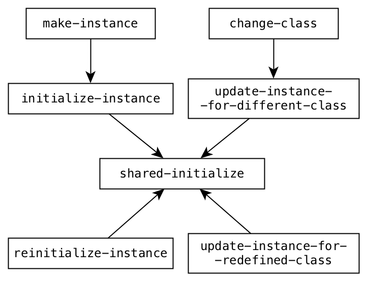
initialize-instance: called bymake-instanceto initialize a just created instance; the user can extend and/or modify the standard initialization by writing specific methods for some classes.reinitialize-instance: called by the user when he wants to "refresh" some instance; sometimes it is the same as initializing from scratch, sometimes not; in the first case it is better to write an appropriateshared-initializemethod; in the second case, the user must write specific methods forreinitialize-instance.change-class: called by the user when the class of an instance is changed; this function asks for a kind of conversion. Normally this function calls the generic functionupdate-instance-for-different-classand the user may write methods for the latter. A simple example follows.defclass: if adefclassis in fact a redefinition of the class, each time an instance of the old version is considered, the generic functionupdate-instance-for-redefined-classis applied, allowing in principle to coherently continue the work.make-instance: the user can also entirely redefine the creation and initialization process.
Writing appropriate methods for these generic functions, the user can freely define the initialization work, clearly distinguishing the various levels from each other; if sufficient, the programmer may partially or totally use the standard style without any further work. You understand that combining these methods with the user-defined class hierarchy, combining also with the various possibilities of auxiliary methods (:before, :after, :around), the user has a fantastically large workspace. However, once this structure is reasonably understood, it is not difficult to be used, and quickly very powerful.
The example of change-class.
The various situations that are met in the artificial simple example of this section around the change-class generic function allow to easily understand the general CLOS organisation of the initialization work.
(DEFCLASS E12 ()
          ((sl1 :initarg :sl1 :reader sl1)
           (sl2 :initarg :sl2 :reader sl2)))
#<STANDARD-CLASS CL-JUPYTER-USER::E12>
(DEFCLASS E13 ()
          ((sl1 :initarg :sl1 :reader sl1)
           (sl3 :initarg :sl3 :reader sl3)))
#<STANDARD-CLASS CL-JUPYTER-USER::E13>
(defvar ins (make-instance 'e12 :sl1 1 :sl2 2))
INS
(change-class ins 'e13)
#<E13 {10055847F3}>
ins
#<E13 {10055847F3}>
(sl1 ins)
1
(sl3 ins)
UNBOUND-SLOT:
  #<UNBOUND-SLOT SL3 {10056EACC3}>
NIL
Ther is no relation at all between both classes E12 and E13; there is a common slot name, namely sl1, but this does not imply any relation between both classes. With an exception, if ever the class of an instance is changed from E12 to E13, this common slot name will be considered by the standard change-class which in fact calls the standard update-instance-for-different-class: this method transmits the slots with the same names in both classes, gives up the other slots in the source instance, and lets unbound the other slots of the target instance. Here, the sl1 slot has been kept, the sl2 slot has been given up, and the sl3 slot in the result is let unbound, which implies the error when this slot is read by the :reader method sl3. Note also the pseudo-new instance is at the same machine address, but the small
invisible steps of the garbage-collector continually modify the actual addresses, which is made obvious by the value of the symbol ins locating our unique but variable instance.
Let us convert again our instance, but with an additional keyword argument.
(change-class ins 'e12 :sl2 22)
#<E12 {10055847F3}>
(sl2 ins)
22
The default methods are sufficient to pass initial arguments to change-class to obtain partial initializations of the new version of the same instance. Let us consider now the situation where for some strange "theoretical" reason, when the class is changed from E12 to E13, the value of the sl3 slot must be computed as the product of the sl2 slot of the source instance multiplied by some number included in the change-class data. This is obtained as follows.
(DEFMETHOD UPDATE-INSTANCE-FOR-DIFFERENT-CLASS :after
           ((source e12) (target e13) &key (multiplier 1))
           (declare (type number multiplier))
           (setf (slot-value target 'sl3)
                 (* (sl2 source) multiplier)))
#<STANDARD-METHOD COMMON-LISP:UPDATE-INSTANCE-FOR-DIFFERENT-CLASS :AFTER (E12 E13) {10059CC1A3}>
(change-class ins 'e13 :multiplier 4)
#<E13 {10055847F3}>
(list (sl1 ins) (sl3 ins))
(1 88)
Because we have used an :after method, the standard primary method is firstly called, solving the sl1 transfer. And after this is done, our auxiliary method works. Note in particular the elegant handling of the extra multiplier argument; because this keyword argument is used in our method, it becomes available for the user when a change-class E12 $\rightarrow$ E13 happens.
We want finally to consider the situation where a conversion E13 $\rightarrow$ E12 must be installed, where the new version of the instance must have both slots redefined to zero. In this case the old version of the instance is useless, so that we can directly obtain this conversion by a change-class method.
(DEFMETHOD CHANGE-CLASS :after ((ins e13) (class (eql 'e12)) &rest rest)
           (declare (ignore rest))
           (setf (slot-value ins 'sl1) 0
                 (slot-value ins 'sl2) 0))
#<STANDARD-METHOD COMMON-LISP:CHANGE-CLASS :AFTER (E13 (EQL E12)) {1005E41C23}>
(change-class ins 'e12)
#<E12 {10055847F3}>
(list (sl1 ins) (sl2 ins))
(0 0)
What typing is.
The small examples of the previous section were artificial, and we want to consider now a plausible situation. We want to use CLOS to implement a simple coherent typing system, allowing the user to simultaneously use arbitrary types and high levels of functional programming, both subjects being furthermore strongly dependent on each other.
What is typing? If a mathematical definition of typing is wished, many definitions are possible, and one of them is to be illustrated by a small CLOS program. Note this new typing system will be installed while the standard one remains active in our environment.
Typing consists in giving the programmer the ability of partial descriptions of his algorithms. Let us call $\mathcal{A}$ the universe of all the machine objects, $\mathcal{A}$ for anything. Any algorithm can be viewed as a map $\mathcal{A}\rightarrow\mathcal{A}$ not everywhere defined. Typically the Euclid algorithm is defined on the set $\mathbb{N}_* \times \mathbb{N}_*$ of pairs of positive integers, and returns such an integer. The set $\mathbb{N}_*$ is a subset of $\mathcal{A}$, and the latter contains also the set $\mathcal{L}$ of lists of any length; among these lists, some of them are made of two positive integers; let us call $\mathcal{L}(\mathbb{N}_* , \mathbb{N}_*)$ the corresponding subtype. The type specification (signature) for the Euclid algorithm $E$ is then $E: \mathcal{L}(\mathbb{N}_* , \mathbb{N}_*) \rightarrow \mathbb{N}_*$.
Speaking so, we have used a few subsets of $\mathcal{A}$. Such a simple example could create some wrong ideas. On one hand, one could think two different types should be disjoint, but it is not the case for $\mathcal{L}$ and $\mathcal{L}(\mathbb{N}_* , \mathbb{N}_*)$. If not disjoint, one could then require one of the considered types is included in the other one; for example $\mathcal{L}(\mathbb{N}_* , \mathbb{N}_*) \subset \mathcal{L}$ and it seems sensible to organize the types as a large oriented graph describing more and more finely the various sets of objects the user works with. Simple typing systems usually are of this sort.
Another idea has a much larger scope; it consists in deciding a type is nothing but some subset of $\mathcal{A}$, where the membership property may be verified by an algorithm. In other words we start only with two predefined types, $\mathcal{A}$ and $\mathcal{B}$; the second one, the Boolean type, has only two objects, $\top$ and $\bot$, implemented in Lisp as the symbols T and NIL. It is then interesting to define a type as an algorithm $\mathcal{A}\rightarrow\mathcal{B}$ everywhere defined; in other words, the algorithm defining a type has the special signature $\mathcal{A}\rightarrow\mathcal{B}$.
This is sufficient in simple programming, but fails as soon as functional programming must be considered. In fact we meet the Russell paradox or if you prefer the Gödel theorem. Let us call $\mathcal{T}$ the type of ... types, that is the set of functional objects $\alpha:\mathcal{A}\rightarrow\mathcal{B}$. Then no algorithm can verify the membership of $\mathcal{T}$! Let us assume $\tau$ is such an algorithm; therefore $\tau:\mathcal{A}\rightarrow\mathcal{B}$ is everywhere defined and $\tau(\alpha) = \top$ if and only if $\alpha$ defines a type, that is, $\alpha:\mathcal{A}\rightarrow\mathcal{B}$ is also everywhere defined. Then one could design the subtype $\mathcal{T}'$ made of the algorithms $\alpha \in \mathcal{T}$ such that $\alpha(\alpha) = \bot$, in other words the type of "typing algorithms" $\alpha$ that are not "element" of the type associated with $\alpha$. It would be easy to write down the algorithm $\tau'$ corresponding to the new type $\mathcal{T}'$:
$$ \begin{array}{rcll} \tau'(\alpha) &=& \mathtt{if}\ \tau(\alpha) &\mathtt{then}\ \mathtt{not}\ \alpha(\alpha)\\ & & & \mathtt{else}\ \bot \end{array} $$
The algorithm $\tau'$ firstly examines whether its argument $\alpha$ is an algorithm $\mathcal{A}\rightarrow\mathcal{B}$; if yes, the algorithm $\alpha$ may work on any object, in particular on itself, and $\tau'$ returns the opposite of $\alpha(\alpha)$; otherwise the answer is negative. Once the algorithm $\tau:\mathcal{A}\rightarrow\mathcal{B}$ is available, then the object $\tau':\mathcal{A}\rightarrow\mathcal{B}$ is available too, but Cantor and Russell remarked there is no possible answer for $\tau'(\tau')$: the answer of $\tau(\tau')$ should certainly be $\top$, so that we obtain the contradictory relation $\tau'(\tau') = \mathtt{not}\ \tau'(\tau')$. Therefore the algorithm $\tau$ may not exist.
The traditional (pseudo-) solution for this difficult problem consists in delaying the examination of the type of functional objects. If an object $\alpha$ is claimed to be an algorithm $\mathcal{T}_1\rightarrow\mathcal{T}_2$, this cannot be verified by a general algorithm; instead, we must wait for an actual run of the algorithm $\alpha$: if the computation of $\alpha(\omega)$ is asked for, some process can then verify the argument $\omega$ is really in the type $\mathcal{T}_1$; if yes the computation of $\alpha(\omega)$ is started and the result $\omega'$ is examined in turn, verifying the relation $\omega' \in\mathcal{T}_2$. In other words it is not possible to verify the type of a functional object in general; the only possible verification consists, each time the algorithm works, in verifying that the argument and the result have the correct type; this "verification" is not at all complete, it can be applied only to a finite number of calls of the algorithm $\alpha$.
This organization must be recursive: the source and/or target types could in turn be functional, so that the verifications $\omega \in \mathcal{T}_1$ and $\omega' \in \mathcal{T}_2$ maybe must also be "delayed" with the meaning just explained. In particular if $\omega$ and $\omega'$ are both functional, then the functional object $\omega$ will probably be used when the object $\omega'$ will work. It is only at this time the correctness of the claimed types for $\omega$, at least for this particular use, may be verified. Examples of this sort are showed in this paper.
In this way, when a whole program is executed, all the particular uses of the functional objects imply that the type of arguments and result are verified, so that when the program is finished, for all the invocations of functional objects, types of input and output are confirmed. Thinking a little about this situation finally leads to the following conclusion: as far as they have been used, the type rules about functional objects have been satisfied for this specific run. A quite satisfactory conclusion.
To illustrate the Common Lisp object system, we take as exercise subject the implementation of such an organization in Common Lisp, using the main components of CLOS.
Classes as structured types.
A class is firstly a structured type. Each instance (element) of a standard class has several slots (components, fields, members), and each slot has various properties described in the definition of the class. The builtin classes, corresponding to old classical types (integers, symbols, ...), are not standard.
The classes are organized in a hierarchical way: a class may be or not a subclass of another one, and this defines an order between the defined classes. This order must be coherent but in general it is not total, that is, for two classes $\mathcal{C}_1$ and $\mathcal{C}_2$, they may or may not be compared. But any class is a subclass of the maximal type~$\mathcal{A}$, which contains any object, in particular the corresponding class object itself; to prove this point, we assign this class object to the symbol universe and verify the object so located is of the type so described; this maximal class $\mathcal{A}$ corresponds to the set (type) $\mathcal{A}$ of the previous section.
(defvar universe (find-class 't))
UNIVERSE
(typep universe universe)
T
The types of the proposed organization for typing in this paper are pointed out by the letters TP only. This is necessary because we have to simultaneously work with three typing systems:
- The old one of Common Lisp, still present in our workspace; we call it the type-system;
- The class-system which is the main constituent of CLOS;
- The theoretical proposal of our exercise; it is called the
TP-system in this text.
In the following, we use a metaobject protocol for CLOS which is not part of the ANSI Common Lisp standard. The SBCL compiler implements this protocol in the
sb-moppackage.
(use-package :sb-mop)
T
The TP-class.
Each TP-type is described by an instance of the TP class now to be defined. We define this class as follows:
(DEFCLASS TP ()
          ((name :type symbol :initarg :name :initform (gensym) :reader name))
          (:metaclass funcallable-standard-class))
#<FUNCALLABLE-STANDARD-CLASS CL-JUPYTER-USER::TP>
At this time, only one slot called name is defined for an instance of TP. Four slot-options have been used with the following meanings:
- The
:typeoption explains thenameslot must contain asymbol; - The
:initargoption says thenameslot may be initialized through the keyword:name; - The
:initformoption says that if thenameslot is not otherwise initialized, it must be automatically initialized by thegensymfunction, a predefined Lisp function which creates from scratch a certainly new symbol; - Finally the
:readeroption asks CLOS to construct a method namednameallowing the user to call this method to obtain the value of the slot.
The :metaclass class option is explained later.
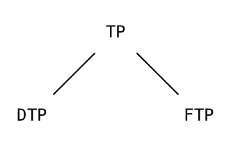
A type descriptor of the TP system is always an instance of the TP-class. The corresponding type is functional or not; if functional the type descriptor is in fact an instance of the FTP class, a subclass of the TP class, else the type descriptor is an instance of the DTP class (discriminant type), another subclass of the TP class. The situation is here particularly simple: a type descriptor is always a TP instance, and in fact always an instance of only one subclass, either FTP, or DTP. Much more complicated situations between classes and subclasses can be designed under CLOS, but this simple situation allows us to show the main points of the nature of CLOS. In other words, the class diagram is this one.
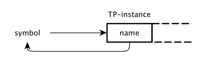
The type descriptor is firstly some TP instance, but it is convenient in this situation to locate the descriptor through a symbol and this is the reason of the name slot: this slot contains the symbol which in principle locates the TP-type descriptor. So that we have two (almost) "symmetric" pointers: the symbol points to the descriptor and the name slot of this descriptor points to this symbol; this is nothing but an explicit C++-this method. If ever the user is not really interested in the symbol, the gensym will automatically generate a symbol for completeness.
The method name may now be applied to a TP-descriptor to obtain the associate symbol.
We have explained in the previous section the role of the print-object generic function. Here, our strategy consists in simply locating TP-types through symbols to be considered as labels, so that it is natural to display such a type by the associate symbol.
(DEFMETHOD PRINT-OBJECT ((tp tp) stream)
           (format stream
                   "#<~S ~S>"
                   (class-name (class-of tp)) (name tp)))
#<STANDARD-METHOD COMMON-LISP:PRINT-OBJECT (TP T) {10064E6213}>
What is finally displayed through the (implicit) call of this method could be for example #<DTP INTEGER>; it is a tradition in Lisp to begin the display of a non-readable object by '#<'; this notion is carefully defined in ANSI Common-Lisp, but it is not the subject of this text. The value of (name tp) is the associate name of the
type-descriptor; the value of (class-of tp) is the class of tp, therefore the class-object DTP or FTP, and
the class-name is the symbol naming this class. We do not want to explain here the technical details of the format Lisp function, which is similar to the traditional printf C function, but fantastically more flexible.
A little earlier the symmetry property between a TP-type descriptor and the symbol locating it was explained. It is a little painful for the user to manage the necessary pointers, but an appropriate method can be used to automate the process during the initialization stage.
(DEFMETHOD INITIALIZE-INSTANCE :after ((tp tp) &rest rest)
           (declare (ignore rest))
           (set (name tp) tp))
#<STANDARD-METHOD COMMON-LISP:INITIALIZE-INSTANCE :AFTER (TP) {10065A4C73}>
The :after qualified method shown above means that after the standard initialization process, something must be done: the symbol in the name slot must be bound to the TP-instance itself.
The DTP-class.
We define now the subclass DTP (discriminant type) of the class TP.
(DEFCLASS DTP (TP)
          ((sub :type list :accessor sub)
           (sup :type list :accessor sup))
          (:metaclass funcallable-standard-class))
#<FUNCALLABLE-STANDARD-CLASS CL-JUPYTER-USER::DTP>
In the first line, the pseudo-argument TP indicates the new class is a subclass of the class TP. Two new slots are defined, so that a DTP-instance will have three slots because of the name slot already defined for a TP-instance:
- The
subslot (sub-types) is a list of the types that are known equal or smaller than the one which is described by theDTP-instance. - The
supslot (super-types) is a list of the types that are known equal or larger than the one which is described by theDTP-instance.
Note that :accessor methods (sub and sup) have been required for the corresponding slots; this means these methods will allow to read the corresponding slot but they can also be used to write it or update it. In fact, these slots must in general be modified after the creation, to maintain the coherence of the TP-system.
We create now the minimal and the maximal type objects of the TP-system, namely the tp-void and tp-any types. A special initialization work is done here because the general initialization process will assume these types are already defined in the environment.
(DEFVAR tp-void (MAKE-INSTANCE 'DTP :name 'tp-void))
TP-VOID
(SETF (sub tp-void) '(tp-void)
      (sup tp-void) '(tp-void tp-any))
(TP-VOID TP-ANY)
(SET-FUNCALLABLE-INSTANCE-FUNCTION tp-void
                                   #'(lambda (obj)
                                             (declare (type t obj) (ignore obj))
                                             (the boolean nil)))
#<FUNCTION (LAMBDA (OBJ) :IN "/home/jovyan/cl-jupyter-master/cl-jupyter.lisp") {100680518B}>
Firstly the DTP-instance to be assigned to the tp-void symbol is created by the call of the generic function make-instance, then the sub and sup slots are defined, and finally, because of the :metaclass class option, it is possible to associate a functional object to this instance, namely the function which always returns nil; this is nothing but the characteristic function of the void type in our environment. Example of use of this function:
(funcall tp-void 'anything)
NIL
Because of the funcall, the functional object associate to the object pointed by the symbol tp-void is called with the symbol anything as argument. Whatever is the argument, the answer is nil. We can verify the pointer symmetry between the name slot and the corresponding symbol:
tp-void
#<DTP TP-VOID>
(name tp-void)
TP-VOID
We do exactly the same work for the tp-any type, perfectly symmetric of the tp-void work.
(DEFVAR tp-any (MAKE-INSTANCE 'DTP :name 'tp-any))
TP-ANY
(SETF (sub tp-any) '(tp-void tp-any)
      (sup tp-any) '(tp-any))
(TP-ANY)
(SET-FUNCALLABLE-INSTANCE-FUNCTION tp-any
                                   #'(lambda (obj)
                                             (declare (type t obj) (ignore obj))
                                             (the boolean t)))
#<FUNCTION (LAMBDA (OBJ) :IN "/home/jovyan/cl-jupyter-master/cl-jupyter.lisp") {100265E9EB}>
(funcall tp-any 'anything)
T
The general process of initialization of a DTP-instance can now be defined. Firstly we need an add-relation function, allowing us to add a new order relation to the environment, something like "integer < number", and all the consequent relations. This function updates the sub and sup slots of the involved DTP-instances with the union Lisp function.
(DEFGENERIC ADD-RELATION (dtp1 dtp2))
#<STANDARD-GENERIC-FUNCTION CL-JUPYTER-USER::ADD-RELATION (0)>
(DEFMETHOD ADD-RELATION ((dtp1 symbol) (dtp2 symbol))
           (the list
                (with-slots (sub) (eval dtp1)
                    (declare (type list sub))
                    (with-slots (sup) (eval dtp2)
                        (declare (type list sup))
                        (dolist (item sub)
                            (declare (type symbol item))
                            (setf (sup (eval item))
                                  (union (sup (eval item)) sup)))
                        (dolist (item sup)
                            (declare (type symbol item))
                            (setf (sub (eval item))
                                  (union (sub (eval item)) sub)))
                        (list dtp1 dtp2)))))
#<STANDARD-METHOD CL-JUPYTER-USER::ADD-RELATION (SYMBOL SYMBOL) {1003AE0103}>
A new :after method can then be defined this time for the DTP-type. Again because this is an :after method, the defined process is added to the standard initialization process, in particular giving the allocation of the instance, the initialization of arguments through initargs and initforms.
(DEFMETHOD INITIALIZE-INSTANCE :after ((dtp dtp)
                                       &key prdc
                                       (dsub '(tp-void))
                                       (dsup '(tp-any)))
           (declare
            (type (function (t) boolean) prdc)
            (type list dsub dsup))
           (with-slots (name sub sup) dtp
               (declare
                (type symbol name)
                (type list sub sup))
               (setf
                sub (union dsub (list name))
                sup (union dsup (list name)))
               (dolist (item dsub)
                   (declare (type symbol item))
                   (add-relation item name))
               (dolist (item dsup)
                   (declare (type symbol item))
                   (add-relation name item)))
           (set-funcallable-instance-function dtp prdc))
#<STANDARD-METHOD COMMON-LISP:INITIALIZE-INSTANCE :AFTER (DTP) {1003EF0A23}>
This method for the generic function initialize-instance uses not only the dtp-instance to be initialized, but also the keyword optional arguments :prdc (predicate), dsub (direct subtypes) and dsup (direct supertypes). This mechanism works as follows: if an initialize-instance method uses a keyword argument, this argument is available to the user when it creates an instance of the corresponding class; usually this argument is used for a small work to be done during the initialization stage. Artificial example:
(defclass cc () ((slot :initarg :slot :reader slot)))
#<STANDARD-CLASS CL-JUPYTER-USER::CC>
(defmethod initialize-instance :after ((cc cc) &key incslot)
    (incf (slot-value cc 'slot) (* 2 incslot)))
#<STANDARD-METHOD COMMON-LISP:INITIALIZE-INSTANCE :AFTER (CC) {10040B1ED3}>
(defvar cc-instance (make-instance 'cc :slot 3 :incslot 5))
CC-INSTANCE
(slot cc-instance)
13
The :slot argument, because it is an :initarg, is used to ordinarily initialize the unique slot named slot of a
c-instance; but the :after initialize-instance method, then adds twice the other keyword argument :incslot.
For the initialization of a dtp-instance, the :prdc argument is used to define the predicate function defining the type, which is associated to the the dtp-instance and used when the dtp-instance is funcalled; the :dsub and :dsup arguments allow the user to give the list of direct sub- and super-types; the method then computes, with the help of add-relation, all the sub- and super-types. If not used, these arguments default to an obvious value.
Let us define the TP-version of the boolean type.
(DEFVAR TP-BOOLEAN
        (MAKE-INSTANCE 'DTP
                       :name 'TP-BOOLEAN
                       :prdc #'(lambda (obj)
                                       (declare (type t obj))
                                       (the boolean
                                            (if (member obj '(nil t))
                                                t nil)))))
TP-BOOLEAN
(funcall tp-boolean 't)
T
(funcall tp-boolean 'true)
NIL
We use now the standard number types tp-number, tp-integer and tp-fixnum to give examples of use of the :dsub and :dsup arguments.
(defvar tp-number (make-instance 'dtp :name 'tp-number :prdc #'numberp))
TP-NUMBER
(defvar tp-fixnum
    (make-instance 'dtp :name 'tp-fixnum
                   :prdc #'(lambda (obj)
                                   (declare (type t obj))
                                   (the boolean
                                        (typep obj 'fixnum)))
                   :dsup '(tp-number)))
TP-FIXNUM
(defvar tp-integer
    (make-instance 'dtp :name 'tp-integer :prdc #'integerp
                   :dsub '(tp-fixnum) :dsup '(tp-number)))
TP-INTEGER
(sup tp-fixnum)
(TP-INTEGER TP-FIXNUM TP-NUMBER TP-ANY)
(funcall tp-fixnum 3)
T
(funcall tp-fixnum 3.3)
NIL
(funcall tp-number 3.3)
T
In particular the relations "tp-fixnum < integer" and "tp-integer < tp-number" have implied "tp-fixnum < tp-number". Note in these examples, the prdc slots for tp-number and tp-integer have been defined through symbols, for example #'numberp points to the functional value of the symbol numberp, in this case a predefined Lisp function examining whether its argument is a number. On the contrary, the prdc slot of the tp-fixnum TP-instance is a function constructed in the call of make-instance.
The user may also construct several new types, and after the fact, explicitly using the add-relation, define the order relations between them.
(defvar t1
    (make-instance 'dtp
                   :name 't1
                   :prdc #'(lambda (obj)
                                   (declare (type t obj))
                                   (the boolean (eql obj 1)))))
T1
(defvar t12
    (make-instance 'dtp
                   :name 't12
                   :prdc #'(lambda (obj)
                                   (declare (type t obj))
                                   (the boolean
                                        (if (member obj '(1 2))
                                            t nil)))))
T12
(defvar t123
    (make-instance 'dtp
                   :name 't123
                   :prdc #'(lambda (obj)
                                   (declare (type t obj))
                                   (the boolean
                                        (if (member obj '(1 2 3))
                                            t nil)))))
T123
(defvar t1234
    (make-instance 'dtp
                   :name 't1234
                   :prdc #'(lambda (obj)
                                   (declare (type t obj))
                                   (the boolean
                                        (if (member obj '(1 2 3 4))
                                            t nil)))))
T1234
We have constructed the types without using the :dsub and :dsup arguments. Then the user can maintain the structure of his type set; the mapcar shows the list of the sup slots of the just defined types.
(mapcar #'sup (list t1 t12 t123 t1234))
((T1 TP-ANY) (T12 TP-ANY) (T123 TP-ANY) (T1234 TP-ANY))
(add-relation 't1 't12)
(T1 T12)
(mapcar #'sup (list t1 t12 t123 t1234))
((T1 T12 TP-ANY) (T12 TP-ANY) (T123 TP-ANY) (T1234 TP-ANY))
(add-relation 't123 't1234)
(T123 T1234)
(mapcar #'sup (list t1 t12 t123 t1234))
((T1 T12 TP-ANY) (T12 TP-ANY) (T123 T1234 TP-ANY) (T1234 TP-ANY))
(add-relation 't12 't123)
(T12 T123)
(mapcar #'sup (list t1 t12 t123 t1234))
((T12 T1 T123 T1234 TP-ANY) (T1234 T123 T12 TP-ANY) (T123 T1234 TP-ANY) (T1234 TP-ANY))
What is striking in such a process is the fact that the order relations must be explained to the machine by the user, again a case of a necessary intuitionistic work! Of course it would be easy to design a simple generator of enumerative types which would itself determine the order relations that are satisfied, but, because of Cantor, Russell and Gödel, this is definitively impossible for general types.
The FTP and SF classes.
Now we process the FTP-class, devoted to the functional types. To simplify the presentation, we consider only the functions $\mathcal{T}_1\rightarrow\mathcal{T}_2$, in other words the functions with exactly one argument. It is easy to prove this is theoretically sufficient, but practically it is not. The standard trick consists in considering a function with two arguments as a function defined for a list of two elements. The further technicalities for the case of an arbitrary number of arguments are far from the subject of this paper, so that we do not want to consider them8.
8 Common Lisp is also there fantastically more advanced than the other current languages: the numerous types of argument transfer that are available give the user a great flexibility to manage the various cases; they are allowed only because of the great mathematical precision of the definition of the language structure.
The FTP-class is defined as follows:
(DEFCLASS FTP (TP)
          ((sorc :type symbol :initarg :sorc :reader sorc)
           (trgt :type symbol :initarg :trgt :reader trgt))
          (:metaclass funcallable-standard-class))
#<FUNCALLABLE-STANDARD-CLASS CL-JUPYTER-USER::FTP>
This time, two slots, sorc (source) and trgt (target), are added to the name slot of the underlying TP-structure; these slots must be two TP-types, in fact two symbols locating them, according to our organization. Note these source and target types can be discriminant or functional.
A functional object will be an instance of the class SF, for safe-function, safe because the types of argument and result are systematically verified when the function is called:
(DEFCLASS SF ()
          ((sorc :type symbol :initarg :sorc :reader sorc)
           (trgt :type symbol :initarg :trgt :reader trgt))
          (:metaclass funcallable-standard-class))
#<FUNCALLABLE-STANDARD-CLASS CL-JUPYTER-USER::SF>
The definition of FTP and SF are almost the same! In the case of an FTP-instance, the associated function will examine whether some object is in this type. In the case of an SF-instance, the associated function will be the functional object itself; the slots sorc and trgt are then additional information about the correct types of argument and result.
To explain the main part of the work to be done now, let us consider a functional type $\mathcal{T}_1\rightarrow\mathcal{T}_2$ and a particular function $f$ declared to be $f:\mathcal{T}'_1\rightarrow\mathcal{T}'_2$; under what circumstances, is this particular $f$ of the functional type $\mathcal{T}_1\rightarrow\mathcal{T}_2$? There is only one solution: we must have the order relations: $\mathcal{T}_1\leq\mathcal{T}'_1$ and $\mathcal{T}_2\leq\mathcal{T}'_2$, and the reader understands now why we took care of these order relations. We therefore need a subtypep Lisp function to compare types. If both arguments are discriminant types, the answer is read in a sup slot; if both arguments are functional, the appropriate comparisons must be applied to the respective sources and targets; if the types are not of the same nature, one being discriminant and the other one being functional, the answer is certainly negative9.
9 It would be easy to work only with (pseudo-) "discriminant" types, even for functional objects, but the organization chosen here makes more obvious the deep difference of nature between both kinds of types; in particular in this way, a DTP-type and an FTP-type can never be compared.
The Lisp translation:
(DEFUN SUBTYPE-P (tp1 tp2)
       (declare (type symbol tp1 tp2))
       (the boolean
            (etypecase (eval tp1)
                (dtp
                 (etypecase (eval tp2)
                     (dtp (if (member tp2 (sup (eval tp1)))
                              t nil))
                     (ftp nil)))
                (ftp
                 (etypecase (eval tp2)
                     (dtp nil)
                     (ftp (and (subtype-p (sorc (eval tp2)) (sorc (eval tp1)))
                               (subtype-p (trgt (eval tp1)) (trgt (eval tp2))))))))))
SUBTYPE-P
We cannot try the subtype-p function until the initialization work for FTP-instances has been completed. Remember in general a TP-instance must also be funcallable to verify the type of any object. The standard initialization work is therefore completed as follows.
(DEFMETHOD INITIALIZE-INSTANCE :after ((ftp ftp) &rest rest)
           (declare (ignore rest))
           (set-funcallable-instance-function ftp
                                              #'(lambda (obj)
                                                        (declare (type t obj))
                                                        (the boolean
                                                             (and (typep obj 'sf)
                                                                  (subtype-p (sorc ftp) (sorc obj))
                                                                  (subtype-p (trgt obj) (trgt ftp)))))))
#<STANDARD-METHOD COMMON-LISP:INITIALIZE-INSTANCE :AFTER (FTP) {1004F65DC3}>
This time the associated function is entirely deduced from the sorc and trgt slots, available after the standard initialization work. You see the only objects of type some FTP-descriptor are SF-instances, and the appropriate order relations must be verified between source, target and the considered functional type. Now we can create a
few FTP-instances and do the obvious tests for subtype-p.
(subtype-p 'tp-fixnum 'tp-integer)
T
(subtype-p 'tp-fixnum 'tp-fixnum)
T
(subtype-p 'tp-integer 'tp-fixnum)
NIL
(defvar fii (make-instance 'ftp
                           :name 'fii
                           :sorc 'tp-integer
                           :trgt 'tp-integer))
FII
(defvar fnf (make-instance 'ftp
                           :name 'fnf
                           :sorc 'tp-number
                           :trgt 'tp-fixnum))
FNF
(subtype-p 'fii 'tp-fixnum)
NIL
(subtype-p 'fii 'fnf)
NIL
(subtype-p 'fnf 'fii)
T
In order to make them work, the initialization of the SF-instances remains to be defined. An SF-instance is funcallable and the associate function will be the ordinary function the user intends to define, with the type verifications automatically added. The Lisp translation:
(DEFMETHOD INITIALIZE-INSTANCE :after ((sf sf) &key f)
           (declare (type (function (t) t) f))
           (set-funcallable-instance-function
            sf
            (with-slots (sorc trgt) sf
                #'(lambda (arg)
                          (declare (type t arg))
                          (unless (funcall (eval sorc) arg)
                              (error "The argument ~S should be of type ~S."
                                     arg sorc))
                          (the t
                               (let ((rslt (funcall f arg)))
                                    (unless (funcall (eval trgt) rslt)
                                        (error "The result ~S should be of type ~S."
                                               rslt trgt))
                                    rslt))))))
#<STANDARD-METHOD COMMON-LISP:INITIALIZE-INSTANCE :AFTER (SF) {10053D2373}>
Note the extra :finitialization argument. An obvious test:
(defvar 2+ (make-instance 'sf
                          :sorc 'tp-integer
                          :trgt 'tp-integer
                          :f #'(lambda (n) (+ n 2))))
2+
(funcall 2+ 5)
7
(funcall 2+ 5.5)
SIMPLE-ERROR:
The argument 5.5 should be of type TP-INTEGER.
NIL
Improvements.
It is a little painful to use the make-instance method with its keywords. Let's use another aspect of the Common Lisp environment, the macro generator to automate the appropriate call to make-instance. Here we detail the work for the creation of SF-instances.
(DEFMACRO MAKE-SF (sorc trgt f)
          `(make-instance 'sf
                          :sorc ,sorc :trgt ,trgt :f ,f))
MAKE-SF
(macroexpand
 '(make-sf 'number 'tp-integer #'(lambda (n) (+ n 5)))))
(MAKE-INSTANCE (QUOTE SF) :SORC (QUOTE NUMBER) :TRGT (QUOTE TP-INTEGER) :F (FUNCTION (LAMBDA (N) (+ N 5))))
(defvar 5+ (make-sf 'tp-number 'tp-integer
                    #'(lambda (n) (+ n 5))))
5+
(funcall 5+ 6)
11
(funcall 5+ 6.5)
SIMPLE-ERROR:
The result 11.5 should be of type TP-INTEGER.
NIL
The defmacro must be considered as defining a source text translator converting a call to make-sf into some
make-instance. The translation mechanism is tested by using the macroexpand Lisp function. Then the 5+ function is really created and then used. This time the error is in the result type.
Constructing the DTP and FTP instances can be processed in the same way.
(DEFMACRO MAKE-DTP (name prdc)
          `(make-instance 'dtp
                          :name ,name :prdc ,prdc))
MAKE-DTP
To explain the coherence of this type system, we add another stage of verification: a discriminant type is essentially a function $\mathcal{A}\rightarrow\mathcal{B}$, so that the functional type of this function should be also verified. Let us solve this challenge. We slightly modify the DTP-initializer.
(DEFMETHOD INITIALIZE-INSTANCE :after ((dtp dtp)
                                       &key prdc
                                       (dsub '(tp-void))
                                       (dsup '(tp-any)))
           (declare
            (type (function (t) boolean) prdc)
            (type list dsub dsup))
           (with-slots (name sub sup) dtp
               (declare
                (type symbol name)
                (type list sub sup))
               (setf
                sub (union dsub (list name))
                sup (union dsup (list name)))
               (dolist (item dsub)
                   (declare (type symbol item))
                   (add-relation item name))
               (dolist (item dsup)
                   (declare (type symbol item))
                   (add-relation name item)))
           (set-funcallable-instance-function dtp
                                              (make-sf 'tp-any 'tp-boolean prdc)))
REDEFINITION-WITH-DEFMETHOD:
  redefining INITIALIZE-INSTANCE :AFTER (#<FUNCALLABLE-STANDARD-CLASS CL-JUPYTER-USER::DTP>) in DEFMETHOD
#<STANDARD-METHOD COMMON-LISP:INITIALIZE-INSTANCE :AFTER (DTP) {1005C5B453}>
As an example, let us consider the frequent case of a user who forgets the positive answer of the member function is not the boolean T:
(member 3 '(1 2 3 4 5))
(3 4 5)
Such a user could erroneously define an enumerative type as follows:
(defvar colors (make-dtp 'colors
                         #'(lambda (obj)
                                   (member obj '(red orange yellow green blue indigo violet)))))
COLORS
(funcall colors 'black)
NIL
(funcall colors 'blue)
SIMPLE-ERROR:
The result (BLUE INDIGO VIOLET) should be of type TP-BOOLEAN.
NIL
and you see the type error ... during the type verification is detected and a clear message is displayed. This cannot be applied to the boolean type itself, because an infinite loop would be generated. You see also in such a case the functional object associated with an instance (DTP) is not purely functional but another (SF)-instance which in turn has an associated functional object.
The function compose.
It is customary in discussions between Lisp and C++ or Java programmers to use the example of the compose function to illustrate how weak C++ is when functional programming is involved; have a look at [CMPS] for the "official" solution in C++ and see how technically difficult it is. Here we give a simple Lisp solution, which furthermore is at once valid for arbitrary data types.
Firstly we construct the pair and any-sf types10:
10 Exercise: a previous version of this paper had the claimed "subtle" definition of the any-sf type: (make-ftp 'any-sf 'tp-void 'tp-any); this really defines a type, but the compose SF-instance would not have the any-sf type, why? Analyzing precisely the difference between both definitions for any-sf is quite interesting and shows that any strict typing system cannot be entirely satisfactory, some freedom must necessarily be given to the programmer; it is exactly the point of view of the Common Lisp designers.
(defvar pair (make-dtp 'pair
                       #'(lambda (obj)
                                 (and (consp obj)
                                      (consp (cdr obj))
                                      (null (cddr obj))))))
PAIR
(defvar any-sf (make-dtp 'any-sf
                         #'(lambda (obj)
                                   (typep obj 'sf))))
ANY-SF
(defvar 2-sf-that-may-be-composed
    (make-dtp '2-sf-that-may-be-composed
              #'(lambda (obj)
                        (and (funcall pair obj)
                             (funcall any-sf (first obj))
                             (funcall any-sf (second obj))
                             (subtype-p (trgt (second obj)) (sorc (first obj)))))))
2-SF-THAT-MAY-BE-COMPOSED
GH: Fix the
make-dtpmacro to accomodate the:dsupparameter!
(setf (sup 2-sf-that-may-be-composed) '(pair))
(PAIR)
(defvar compose
    (make-sf '2-sf-that-may-be-composed 'any-sf
             #'(lambda (arg)
                       (let ((sf2 (first arg))
                             (sf1 (second arg)))
                            (make-sf (sorc sf1) (trgt sf2)
                                     #'(lambda (arg)
                                               (funcall sf2 (funcall sf1 arg))))))))
COMPOSE
(defvar 4+ (funcall compose (list 2+ 2+)))
4+
(funcall 4+ 5)
9
(funcall 4+ 5.5)
SIMPLE-ERROR:
The argument 5.5 should be of type TP-INTEGER.
NIL
A more subtle example: the composed function is in the right type with respect the argument, but a used function is not.
(defvar 3/2+ (make-sf 'tp-integer 'tp-integer
                      #'(lambda (x) (+ x 3/2))))
3/2+
(defvar 3+ (funcall compose (list 3/2+ 3/2+)))
3+
(funcall 3+ 6)
SIMPLE-ERROR:
The result 15/2 should be of type TP-INTEGER.
NIL
The last type-error example; this time, the compose function itself observes its argument does not have the required type.
(funcall compose (list compose compose))
SIMPLE-ERROR:
The argument (#<SF {10061D8A3B}> #<SF {10061D8A3B}>) should be of type 2-SF-THAT-MAY-BE-COMPOSED.
NIL
CLOS and Mathematical Structures.
We give a small example to explain how CLOS can easily be used to implement the classical mathematical structures. Most often, an object of some type in mathematics is a structure with several components, frequently of functional nature. In this small presentation, we consider the case of a user who wants to handle sets, magmas, associative magmas and monoids; these simple particular cases are sufficient to understand how CLOS gives the right tools to process mathematical structures. In the following section, we will describe how these simple methods have been used in [DRSS] to implement the main structures of Algebraic Topology such as chain complexes, simplicial sets, simplicial groups, Hopf algebras, and also the various morphisms between these objects.
Sets.
We define a /SET/ class whose instances correspond to the sets of the classical set theory.
(DEFCLASS /SET/ ()
          ((name :type symbol :initarg :name :initform (gensym) :reader name)
           (prdcf :type function :initarg :prdcf :reader prdcf)
           (cmprf :type function :initarg :cmprf :reader cmprf)))
#<STANDARD-CLASS CL-JUPYTER-USER::/SET/>
In this organization, a set is made of three slots. The name slot has the same role as for the types of the previous section: it is only an auxiliary tool to locate easily the sets; the slot contains the symbol that locates the set, and we automate this organization:
(DEFMETHOD SHARED-INITIALIZE :after ((set /set/) slot-names &rest rest)
           (declare (ignore slot-names rest))
           (set (name set) set))
#<STANDARD-METHOD COMMON-LISP:SHARED-INITIALIZE :AFTER (/SET/ T) {10066AA863}>
The appropriate print-object method; when a set or an object of a subclass will be displayed, the output will show the corresponding class and the name:
(DEFMETHOD PRINT-OBJECT ((set /set/) stream)
           (declare (type stream stream))
           (format stream "#<~S ~S>" (class-name (class-of set)) (name set))
           (the /set/ set))
#<STANDARD-METHOD COMMON-LISP:PRINT-OBJECT (/SET/ T) {10067EC5B3}>
The second slot of a set, namely the prdcf slot (predicate-function), contains a function which can be called to examine whether some arbitrary object is an element of the set. In order to use this slot easily, we define two functions, owns and in; the first one may answer yes or no, that is, t or nil; and the second one generates an error if the membership relation is not satisfied12.
12 The sections bout our two main didactical examples, typing and mathematical categories, are entirely independent; but the lucid reader will observe the root class of the second application, namely the /set/ class, can after all be also considered as a typing system in a mathematical context!
(DEFUN OWNS (set obj)
       (declare
        (type /set/ set)
        (type t obj))
       (the boolean
            (funcall (prdcf set) obj)))
OWNS
(DEFUN IN (set obj)
       (declare
        (type /set/ set)
        (type t obj))
       (if (funcall (prdcf set) obj)
           obj
           (error "The object ~S is not in ~S."
                  obj set)))
IN
The explanation of the third slot cmpr is given a little later; we construct the set N of non-negative integers.
(defvar N
    (MAKE-INSTANCE '/set/
                   :name 'N
                   :prdcf #'(lambda (obj)
                                    (declare (type t obj))
                                    (the boolean
                                         (and (integerp obj)
                                              (>= obj 0))))
                   :cmprf #'=))
N
The symbol N locates the constructed set
N
#</SET/ N>
and the function owns allows the user to examine the membership relation:
(owns N +1)
T
(owns N -1)
NIL
The cmprf slot is essential in this context. There are frequently strong differences between an element of a set as thought by the mathematician and its possible machine representations, the s being important. The notion of equality in mathematics is "primitive" and rarely logically considered by mathematicians. On the contrary, this notion is crucial in Computer Science, and Common Lisp is by far the most precise language from this point of view13. Here, we want to let the user freely decide how equality is defined between the elements of his sets, and this is the role of the cmprf slot (comparison function). For example, the comparison between elements in the set N is done by the Lisp predefined function #'=, in particular appropriate to compare integers. Again we define a function cmpr to easily use the cmprf slot of a set.
13 In particular all the standard predefined Lisp functions allow the user to freely define the equality relation to be used for every particular call.
(DEFUN ELT-CMPR (set elmn1 elmn2)
       (declare
        (type /set/ set)
        (type t elmn1 elmn2))
       (the boolean
            (funcall (cmprf set)
                     (in set elmn1) (in set elmn2))))
ELT-CMPR
Note the use of the in function to verify that the compared elements are really in the considered set. Now we can compare two elements of N.
(elt-cmpr N 4 9)
NIL
(elt-cmpr N 4 -9)
SIMPLE-ERROR:
The object -9 is not in #</SET/ N>.
NIL
Let us construct now the set Z/5, that is the set of integers modulo 5. In our context, the most elegant method to implement this set consists in admitting a representation of an element of Z/5 by an arbitrary integer, possibly negative or > 4, and to define the comparison with the help of the mod function, a predefined Lisp function.
(defvar Z/5
    (MAKE-INSTANCE '/SET/
                   :name 'Z/5
                   :prdcf #'integerp
                   :cmprf #'(lambda (elmn1 elmn2)
                                    (= 0 (mod (- elmn1 elmn2) 5)))))
Z/5
(elt-cmpr Z/5 4 9)
T
This time the comparison between 4 and 9 is positive: these machine integers are different representations of the same mathematical object. You will understand that it is easy in this framework to define quotient sets.
Magmas.
A magma is a set provided with a law of composition without any particular required property. It is a set with an additional ingredient, a function able to work on two elements of the magma and returning another element, their composition according the composition law. It is natural in this context to define the magma subclass of the /set/ class; any magma instance is a set with a further slot, the lawf slot.
(DEFCLASS MAGMA (/set/)
          ((lawf :type function :initarg :lawf :reader lawf)))
#<STANDARD-CLASS CL-JUPYTER-USER::MAGMA>
Again a function is added to the environment allowing the user to easily refer the lawf slot of a magma.
(DEFGENERIC LAW (magma &rest rest))
#<STANDARD-GENERIC-FUNCTION CL-JUPYTER-USER::LAW (0)>
(DEFMETHOD LAW ((magma magma) &rest rest)
           (case (length rest)
               (1 (in magma (first rest)))
               (2 (in magma
                      (funcall (lawf magma)
                               (in magma (first rest))
                               (in magma (second rest)))))
               (otherwise
                (error "Non-correct arguments in:~@
                       (LAW ~S~{ ~S~})." magma rest))))
#<STANDARD-METHOD CL-JUPYTER-USER::LAW (MAGMA) {1003C2ADC3}>
We intend in general to allow the user to refer the law defining a magma with an arbitrary number of elements, at least if this makes sense. In such a case, CLOS allows the user to define a generic function, here the law generic function, with one mandatory argument, called here magma and any number of other arguments put together in a list reachable through the symbol rest14. The ingredient (magma magma) in the parameter list has two meanings: the first magma names the first parameter, and the second magma explains the corresponding argument must be of class magma, otherwise the method is not applicable.
14 More precisely, the symbol &rest marks in the parameter list a new zone, in this case with a symbol locating the "other" arguments; the Lisp programmer almost always chooses the symbol rest to locate this list.
For a magma without any further claimed property, it is sensible to allow one argument, and then this argument is returned, or two arguments and then the product of these arguments according to the composition law is returned.
Otherwise an error message is displayed. Note how the in function is used to verify the correct type of the arguments.
We have defined the set N and it is possible to transform it now into a magma. Note how the standard initialization process of an instance allows the user to obtain such a conversion without any further work.
(change-class N 'magma
              :lawf #'(lambda (n1 n2)
                              (* n1 (- n2 3))))
#<MAGMA N>
The law which is defined is $(n_1,n_2) \mapsto n_1(n_2-3)$. The obvious trials:
(law N 4 5)
8
(law N 4 -5)
SIMPLE-ERROR:
The object -5 is not in #<MAGMA N>.
NIL
(law N 1 0)
SIMPLE-ERROR:
The object -3 is not in #<MAGMA N>.
NIL
(law N 4)
4
(law N 4 5 6)
SIMPLE-ERROR:
Non-correct arguments in:
(LAW #<MAGMA N> 4 5 6).
NIL
The constructed magma in fact is not correct; let us construct a classical correct one:
(defvar Q
    (make-instance 'magma
                   :name 'Q
                   :prdcf #'rationalp
                   :cmprf #'=
                   :lawf #'+))
Q
(law Q 3/2 2/3)
13/6
(law Q 3/2 2/3 4/5)
SIMPLE-ERROR:
Non-correct arguments in:
(LAW #<MAGMA Q> 3/2 2/3 4/5).
NIL
This is simply the set Q of rationals equipped with the standard addition law. The last result is not satisfactory: the law is associative and it should be possible to make operate this law on an arbitrary number of arguments. The solution consists in defining a new class A-MAGMA (associative magma). There is no new slot in this class: membership of the new class only means the object, some magma, has an associative law.
(DEFCLASS A-MAGMA (magma) ())
#<STANDARD-CLASS CL-JUPYTER-USER::A-MAGMA>
But this new class may be used to define a new method for the generic function law; in this new case, an arbitrary positive number of arguments can be used. A simple recursive process defines the new method from the old one: if the argument number is three or more, the computation is decomposed, otherwise the next method is called; the law is associative and this definition is coherent.
(DEFMETHOD LAW ((a-magma a-magma) &rest rest)
           (if (> (length rest) 2)
               (law a-magma
                    (in a-magma (first rest))
                    (apply #'law a-magma (rest rest)))
               (call-next-method)))
#<STANDARD-METHOD CL-JUPYTER-USER::LAW (A-MAGMA) {100432C8D3}>
You see in particular how the very basic Lisp function apply allows to recall the same method with one argument removed. We inform now the environment that our magma Q is associative:
(change-class Q 'a-magma)
#<A-MAGMA Q>
which allows us to compute the composition in Q of an arbitrary number of elements. Because the magma method will eventually be called, a possible type fault is intercepted.
(law Q 1/2 2/3 3/4 4/5)
163/60
(law Q 1/2 2/3 0.75 4/5)
SIMPLE-ERROR:
The object 0.75 is not in #<A-MAGMA Q>.
NIL
Monoids.
And the process can be continued for ever and ever, allowing the user to enrich as far as necessary the considered mathematical structures. Here, the following step consists in considering the structure of monoids. A monoid is an
associative magma with a unit. Only a unit slot is to be added to the a-magma structure. It is impossible in general to verify the claimed unit $e$ satisfies the required property, but however the property $e\ast e = e$ can be tested; doing this test through a shared-initialize method allows it to be used in a make-instance, or in a change-class, or in a reinitialize-instance as well. The membership of the monoid may be also tested.
(DEFCLASS MONOID (a-magma)
          ((unit :initarg :unit :reader unit)))
#<STANDARD-CLASS CL-JUPYTER-USER::MONOID>
(DEFMETHOD SHARED-INITIALIZE :after ((monoid monoid) slot-names &rest rest)
           (declare (ignore rest))
           (let ((unit (unit monoid)))
                (unless (owns monoid unit)
                    (error "Sorry, the claimed unit ~S is not in ~S."
                           unit monoid))
                (unless (elt-cmpr monoid unit (law monoid unit unit))
                    (error "Sorry, ~S does not look like a unit in ~S."
                           unit monoid))))
#<STANDARD-METHOD COMMON-LISP:SHARED-INITIALIZE :AFTER (MONOID T) {10045E20C3}>
(change-class Q 'monoid :unit 1)
SIMPLE-ERROR:
Sorry, 1 does not look like a unit in #<MONOID Q>.
NIL
(reinitialize-instance Q :unit 0)
#<MONOID Q>
Note the error about the unit is intercepted after the standard initialization process, so that our Q is then become a monoid, as observed in the error message, but a wrong monoid; it is natural in this situation to use reinitialize-instance to redefine the object. A little more sophisticated use of :around methods would allow us to verify the coherence before changing class, and to refuse it if detected non-coherent.
It is interesting to convert Z/5, currently a set, into a monoid with the unit 10. Why not?
(change-class Z/5 'monoid
              :lawf #'+
              :unit 10)
#<MONOID Z/5>
(elt-cmpr Z/5 10 (law Z/5 10 10))
T
In a monoid, the composition law may logically be called for zero argument; in this case, the unit is the result. A new method for the generic function law is therefore stacked.
(DEFMETHOD LAW ((monoid monoid) &rest rest)
           (if (= 0 (length rest))
               (unit monoid)
               (call-next-method)))
#<STANDARD-METHOD CL-JUPYTER-USER::LAW (MONOID) {10049FA4B3}>
(list (law Q) (law Z/5))
(0 10)
This looks a little artificial because (law Q) and (unit Q) are in fact synonymous, but think of the frequent case where you have to process a statement like (apply #'law Q some-list) where the last argument is a computed list, which could be sometimes empty; with our new monoid method for the law generic function, even if the value of some-list is the empty list, the correct process is applied.
What about the morphisms?
So far we have only worked with the objects of the mathematical categories of sets, magmas, associative magmas, monoids. What about the morphisms? The solution is easy, but needs a little lucidity about the usual compatibility properties with ambient structures. We only sketch a possible solution, the expansion of which being obvious.
The root of our classes of morphisms is the class of morphisms between sets.
(DEFCLASS SET-MRPH ()
          ((sorc :type set :initarg :sorc :reader sorc)
           (trgt :type set :initarg :trgt :reader trgt)
           (f :type function :initarg :f :reader f)))
A set-mrph instance is essentially a source, some set, a target, some set, and a function mapping any object of the source to an object of the target. Again the standard functional properties of Common Lisp give the developper the right environment. We could also hide the f slot into the special hidden functional slot of a funcallable instance, as we did for the TP-instances in Section 3; it is only a question of taste.
We need something to be able to "funcall" a set-mrph:
(DEFUN ? (mrph elmn)
    (...
         code which:
             1) verifies elmn is in the source of mrph;
             2) applies the f slot of mrph to elmn to compute the image;
             3) verifies this image is in the target of mrph;
             4) returns the image.
    ))

(? some-set-mrph some-source-element)
Now a magma-morphism is nothing but a set-morphism satisfying the standard compatibility properties with the magma structures of source and target. So that:
(DEFCLASS MAGMA-MRPH (set-mrph) ())
and the same for a-magma-mrph, monoid-mrph and so on. Note this organization allows the user to clearly distinguish a
set-morphism between magmas from a magma-morphism between the same magmas; in the first case the compatibility properties are not satisfied or optional; in the second case the compatibility properties are assumed satisfied. Such morphisms are intensively used in the Kenzo program and considered in the following section.
What about functors?
Working with categories, the mathematician inevitably will have to work with functors. In this organisation a tower of compatible functors is nothing but one generic function with various methods corresponding to the different cases. For example the cartesian product functor is defined for sets, magmas, associative magmas, monoids, and many other categories. It is sufficient to implement all these functors in one generic function, as follows.
(DEFGENERIC PRODUCT (set1 set2))
#<STANDARD-GENERIC-FUNCTION CL-JUPYTER-USER::PRODUCT (0)>
(DEFMETHOD PRODUCT ((set1 /set/) (set2 /set/))
           (make-instance '/set/
                          :name (intern (format nil "~S-PRDC-~S" (name set1) (name set2)))
                          :prdcf #'(lambda (obj)
                                           (declare (type t obj))
                                           (the boolean
                                                (and (listp obj)
                                                     (= 2 (length obj))
                                                     (owns set1 (first obj))
                                                     (owns set2 (second obj)))))
                          :cmprf #'(lambda (pair1 pair2)
                                           (declare (type list pair1 pair2))
                                           (the boolean
                                                (and (elt-cmpr set1 (first pair1) (first pair2))
                                                     (elt-cmpr set2 (second pair1) (second pair2)))))))
#<STANDARD-METHOD CL-JUPYTER-USER::PRODUCT (/SET/ /SET/) {1004C8F443}>
(product N Z/5)
#</SET/ N-PRDC-Z/5>
(elt-cmpr N-prdc-Z/5 '(4 5) '(9 5))
NIL
(elt-cmpr N-prdc-Z/5 '(4 5) '(4 10))
T
(elt-cmpr N-prdc-Z/5 '(4 5) '(-4 10))
SIMPLE-ERROR:
The object (-4 10) is not in #</SET/ N-PRDC-Z/5>.
NIL
You see how clear and natural is the code of the product method. It is only a question of constructing the appropriate prdcf and cmprf slots, some functions, from the corresponding slots of the arguments set1 and set2; the process is always the same, so that the Lisp closures, a subtle notion not available in C++ or Java15, give the user the natural tool, even he does not know exactly what a closure is!
15 available in Maple since the Release 5, but no OOP in Maple...
For the richer structures of magma, a-magma and monoid, it is sufficient to write down new specific methods for the same generic function, defining the additional work to be done, using the previous work thanks to call-next-method.
(DEFMETHOD PRODUCT ((magma1 magma) (magma2 magma))
           (change-class (call-next-method) 'magma
                         :lawf #'(lambda (pair1 pair2)
                                         (list
                                          (law magma1 (first pair1) (first pair2))
                                          (law magma2 (second pair1) (second pair2))))))
#<STANDARD-METHOD CL-JUPYTER-USER::PRODUCT (MAGMA MAGMA) {100515B453}>
(DEFMETHOD PRODUCT ((magma1 a-magma) (magma2 a-magma))
           (change-class (call-next-method) 'a-magma))
#<STANDARD-METHOD CL-JUPYTER-USER::PRODUCT (A-MAGMA A-MAGMA) {1005372D83}>
(DEFMETHOD PRODUCT ((monoid1 monoid) (monoid2 monoid))
           (change-class (call-next-method) 'monoid
                         :unit (list (unit monoid1) (unit monoid2))))
#<STANDARD-METHOD CL-JUPYTER-USER::PRODUCT (MONOID MONOID) {1005594E23}>
(DEFVAR Q2 (product Q Q))
Q2
(DEFVAR Q4 (product Q2 Q2))
Q4
(law Q4 '((1/2 2/3) (3/4 4/5))
     '((5/6 6/7) (7/8 8/9)))
((4/3 32/21) (13/8 76/45))
(unit Q4)
((0 0) (0 0))
Note also the applicability rule for methods of a generic function implies the product of a monoid by a magma, for example, will fortunately be a magma.
(product Q N)
#<MAGMA Q-PRDC-N>
CLOS and the Kenzo program.
Some of the comments in this section apply to an older Kenzo version. They are called out whenever there's a difference in implementation and behavior with the newer version.
The Kenzo program is the first significant machine program about classical Algebraic Topology. It is not only a program implementing various known algorithms; new methods have been developped to transform the main "tools" of Algebraic Topology, mainly the spectral sequences, not at all algorithmic in the traditionnal organisation, into actual computing methods.
An example of Kenzo work.
Let us show a simple example to illustrate which is possible with this program. The homology group $H_5 \Omega^3 \mathrm{Moore}(\mathbb{Z}_2,4)$16 is "in principle" reachable thanks to old methods, see [CRML], but experience shows even the most skilful topologists meet some difficulties to determine it, see [RBSR6][SRGR5]. With the Kenzo program, you construct the Moore space.
16 The space $\mathrm{Moore}(\mathbb{Z}_2,4)$ is a "canonical" space having only non-trivial homology in dimension~4, namely $\mathbb{Z}_2$, and $\Omega^3\mathrm{Moore}(\mathbb{Z}_2,4)$, its third loop space, is the space of continuous maps from the 3-sphere~$S^3$ to this Moore space; the challenge is to determine the fifth homology group of this functional space.
(cat-init)
---done---
NIL
(def m4 (moore 2 4))
[K1 Simplicial-Set]
The program returns the Kenzo-object #1, a simplicial set, that is, a combinatorial version of the Moore space which is asked for, and this object is assigned to the symbol m4. Then you construct the third loop-space of this Moore space.
(def o3m4 (loop-space m4 3))
[K30 Simplicial-Group]
The combinatorial version of the loop space is highly infinite: it is a combinatorial version of the space of continuous maps $S^3 \rightarrow \mathrm{Moore}(\mathbb{Z}_2,4)$ but functionnally coded as a small set of functions
in a simplicial-group object, that is, a simplicial set with an added group structure compatible with the simplicial structure. Finally the fifth homology-group is asked for.
(homology o3m4 5)
Computing boundary-matrix in dimension 5.
Rank of the source-module : 23.


;; Clock -> 2017-02-26, 2h 19m 16s.
Computing the boundary of the generator 1/23 (dimension 5) :
<<AlLp[5 <<AlLp[6 <<AlLp[3 M4][4 N5]>>]>>]>>
End of computing.


;; Clock -> 2017-02-26, 2h 19m 16s.
Computing the boundary of the generator 2/23 (dimension 5) :
<<AlLp[5 <<AlLp[6 <<AlLp[4 N5][3 M4]>>]>>]>>
End of computing.


;; Clock -> 2017-02-26, 2h 19m 16s.
Computing the boundary of the generator 3/23 (dimension 5) :
<<AlLp[5 <<AlLp[3 <<AlLp[4 N5]>>][3 <<AlLp[4 N5]>>]>>]>>
End of computing.


;; Clock -> 2017-02-26, 2h 19m 16s.
Computing the boundary of the generator 4/23 (dimension 5) :
<<AlLp[5 <<AlLp[2 <<AlLp[3 M4]>>][2 <<AlLp[3 M4]>>][2 <<AlLp[3 M4]>>]>>]>>
End of computing.


;; Clock -> 2017-02-26, 2h 19m 16s.
Computing the boundary of the generator 5/23 (dimension 5) :
<<AlLp[1 <<AlLp[2 <<AlLp[3 M4]>>]>>][4 <<AlLp[5 <<AlLp[3 M4][3 M4]>>]>>]>>
End of computing.


;; Clock -> 2017-02-26, 2h 19m 16s.
Computing the boundary of the generator 6/23 (dimension 5) :
<<AlLp[1 <<AlLp[2 <<AlLp[3 M4]>>]>>][4 <<AlLp[2 <<AlLp[3 M4]>>][3 <<AlLp[4 N5]>>]>>]>>
End of computing.


;; Clock -> 2017-02-26, 2h 19m 16s.
Computing the boundary of the generator 7/23 (dimension 5) :
<<AlLp[1 <<AlLp[2 <<AlLp[3 M4]>>]>>][4 <<AlLp[3 <<AlLp[4 N5]>>][2 <<AlLp[3 M4]>>]>>]>>
End of computing.


;; Clock -> 2017-02-26, 2h 19m 16s.
Computing the boundary of the generator 8/23 (dimension 5) :
<<AlLp[2 <<AlLp[3 <<AlLp[4 N5]>>]>>][3 <<AlLp[2 <<AlLp[3 M4]>>][2 <<AlLp[3 M4]>>]>>]>>
End of computing.


;; Clock -> 2017-02-26, 2h 19m 16s.
Computing the boundary of the generator 9/23 (dimension 5) :
<<AlLp[3 <<AlLp[2 <<AlLp[3 M4]>>][2 <<AlLp[3 M4]>>]>>][2 <<AlLp[3 <<AlLp[4 N5]>>]>>]>>
End of computing.


;; Clock -> 2017-02-26, 2h 19m 16s.
Computing the boundary of the generator 10/23 (dimension 5) :
<<AlLp[4 <<AlLp[5 <<AlLp[3 M4][3 M4]>>]>>][1 <<AlLp[2 <<AlLp[3 M4]>>]>>]>>
End of computing.


;; Clock -> 2017-02-26, 2h 19m 16s.
Computing the boundary of the generator 11/23 (dimension 5) :
<<AlLp[4 <<AlLp[2 <<AlLp[3 M4]>>][3 <<AlLp[4 N5]>>]>>][1 <<AlLp[2 <<AlLp[3 M4]>>]>>]>>
End of computing.


;; Clock -> 2017-02-26, 2h 19m 16s.
Computing the boundary of the generator 12/23 (dimension 5) :
<<AlLp[4 <<AlLp[3 <<AlLp[4 N5]>>][2 <<AlLp[3 M4]>>]>>][1 <<AlLp[2 <<AlLp[3 M4]>>]>>]>>
End of computing.


;; Clock -> 2017-02-26, 2h 19m 16s.
Computing the boundary of the generator 13/23 (dimension 5) :
<<AlLp[1 <<AlLp[2 <<AlLp[3 M4]>>]>>][1 <<AlLp[2 <<AlLp[3 M4]>>]>>][3 <<AlLp[2 <<AlLp[3 M4]>>][2 <<AlLp[3 M4]>>]>>]>>
End of computing.


;; Clock -> 2017-02-26, 2h 19m 16s.
Computing the boundary of the generator 14/23 (dimension 5) :
<<AlLp[1 <<AlLp[2 <<AlLp[3 M4]>>]>>][2 <<AlLp[3 <<AlLp[4 N5]>>]>>][2 <<AlLp[3 <<AlLp[4 N5]>>]>>]>>
End of computing.


;; Clock -> 2017-02-26, 2h 19m 16s.
Computing the boundary of the generator 15/23 (dimension 5) :
<<AlLp[1 <<AlLp[2 <<AlLp[3 M4]>>]>>][3 <<AlLp[2 <<AlLp[3 M4]>>][2 <<AlLp[3 M4]>>]>>][1 <<AlLp[2 <<AlLp[3 M4]>>]>>]>>
End of computing.


;; Clock -> 2017-02-26, 2h 19m 16s.
Computing the boundary of the generator 16/23 (dimension 5) :
<<AlLp[2 <<AlLp[3 <<AlLp[4 N5]>>]>>][1 <<AlLp[2 <<AlLp[3 M4]>>]>>][2 <<AlLp[3 <<AlLp[4 N5]>>]>>]>>
End of computing.


;; Clock -> 2017-02-26, 2h 19m 16s.
Computing the boundary of the generator 17/23 (dimension 5) :
<<AlLp[2 <<AlLp[3 <<AlLp[4 N5]>>]>>][2 <<AlLp[3 <<AlLp[4 N5]>>]>>][1 <<AlLp[2 <<AlLp[3 M4]>>]>>]>>
End of computing.


;; Clock -> 2017-02-26, 2h 19m 16s.
Computing the boundary of the generator 18/23 (dimension 5) :
<<AlLp[3 <<AlLp[2 <<AlLp[3 M4]>>][2 <<AlLp[3 M4]>>]>>][1 <<AlLp[2 <<AlLp[3 M4]>>]>>][1 <<AlLp[2 <<AlLp[3 M4]>>]>>]>>
End of computing.


;; Clock -> 2017-02-26, 2h 19m 16s.
Computing the boundary of the generator 19/23 (dimension 5) :
<<AlLp[1 <<AlLp[2 <<AlLp[3 M4]>>]>>][1 <<AlLp[2 <<AlLp[3 M4]>>]>>][1 <<AlLp[2 <<AlLp[3 M4]>>]>>][2 <<AlLp[3 <<AlLp[4 N5]>>]>>]>>
End of computing.


;; Clock -> 2017-02-26, 2h 19m 16s.
Computing the boundary of the generator 20/23 (dimension 5) :
<<AlLp[1 <<AlLp[2 <<AlLp[3 M4]>>]>>][1 <<AlLp[2 <<AlLp[3 M4]>>]>>][2 <<AlLp[3 <<AlLp[4 N5]>>]>>][1 <<AlLp[2 <<AlLp[3 M4]>>]>>]>>
End of computing.


;; Clock -> 2017-02-26, 2h 19m 16s.
Computing the boundary of the generator 21/23 (dimension 5) :
<<AlLp[1 <<AlLp[2 <<AlLp[3 M4]>>]>>][2 <<AlLp[3 <<AlLp[4 N5]>>]>>][1 <<AlLp[2 <<AlLp[3 M4]>>]>>][1 <<AlLp[2 <<AlLp[3 M4]>>]>>]>>
End of computing.


;; Clock -> 2017-02-26, 2h 19m 16s.
Computing the boundary of the generator 22/23 (dimension 5) :
<<AlLp[2 <<AlLp[3 <<AlLp[4 N5]>>]>>][1 <<AlLp[2 <<AlLp[3 M4]>>]>>][1 <<AlLp[2 <<AlLp[3 M4]>>]>>][1 <<AlLp[2 <<AlLp[3 M4]>>]>>]>>
End of computing.


;; Clock -> 2017-02-26, 2h 19m 16s.
Computing the boundary of the generator 23/23 (dimension 5) :
<<AlLp[1 <<AlLp[2 <<AlLp[3 M4]>>]>>][1 <<AlLp[2 <<AlLp[3 M4]>>]>>][1 <<AlLp[2 <<AlLp[3 M4]>>]>>][1 <<AlLp[2 <<AlLp[3 M4]>>]>>][1 <<AlLp[2 <<AlLp[3 M4]>>]>>]>>
End of computing.


Computing boundary-matrix in dimension 6.
Rank of the source-module : 53.


;; Clock -> 2017-02-26, 2h 19m 16s.
Computing the boundary of the generator 1/53 (dimension 6) :
<<AlLp[6 <<AlLp[7 <<AlLp[4 N5][4 N5]>>]>>]>>
End of computing.


;; Clock -> 2017-02-26, 2h 19m 16s.
Computing the boundary of the generator 2/53 (dimension 6) :
<<AlLp[6 <<AlLp[2 <<AlLp[3 M4]>>][5 <<AlLp[3 M4][3 M4]>>]>>]>>
End of computing.


;; Clock -> 2017-02-26, 2h 19m 16s.
Computing the boundary of the generator 3/53 (dimension 6) :
<<AlLp[6 <<AlLp[5 <<AlLp[3 M4][3 M4]>>][2 <<AlLp[3 M4]>>]>>]>>
End of computing.


;; Clock -> 2017-02-26, 2h 19m 17s.
Computing the boundary of the generator 4/53 (dimension 6) :
<<AlLp[6 <<AlLp[2 <<AlLp[3 M4]>>][2 <<AlLp[3 M4]>>][3 <<AlLp[4 N5]>>]>>]>>
End of computing.


;; Clock -> 2017-02-26, 2h 19m 17s.
Computing the boundary of the generator 5/53 (dimension 6) :
<<AlLp[6 <<AlLp[2 <<AlLp[3 M4]>>][3 <<AlLp[4 N5]>>][2 <<AlLp[3 M4]>>]>>]>>
End of computing.


;; Clock -> 2017-02-26, 2h 19m 17s.
Computing the boundary of the generator 6/53 (dimension 6) :
<<AlLp[6 <<AlLp[3 <<AlLp[4 N5]>>][2 <<AlLp[3 M4]>>][2 <<AlLp[3 M4]>>]>>]>>
End of computing.


;; Clock -> 2017-02-26, 2h 19m 17s.
Computing the boundary of the generator 7/53 (dimension 6) :
<<AlLp[1 <<AlLp[2 <<AlLp[3 M4]>>]>>][5 <<AlLp[6 <<AlLp[3 M4][4 N5]>>]>>]>>
End of computing.


;; Clock -> 2017-02-26, 2h 19m 17s.
Computing the boundary of the generator 8/53 (dimension 6) :
<<AlLp[1 <<AlLp[2 <<AlLp[3 M4]>>]>>][5 <<AlLp[6 <<AlLp[4 N5][3 M4]>>]>>]>>
End of computing.


;; Clock -> 2017-02-26, 2h 19m 17s.
Computing the boundary of the generator 9/53 (dimension 6) :
<<AlLp[1 <<AlLp[2 <<AlLp[3 M4]>>]>>][5 <<AlLp[3 <<AlLp[4 N5]>>][3 <<AlLp[4 N5]>>]>>]>>
End of computing.


;; Clock -> 2017-02-26, 2h 19m 17s.
Computing the boundary of the generator 10/53 (dimension 6) :
<<AlLp[1 <<AlLp[2 <<AlLp[3 M4]>>]>>][5 <<AlLp[2 <<AlLp[3 M4]>>][2 <<AlLp[3 M4]>>][2 <<AlLp[3 M4]>>]>>]>>
End of computing.


;; Clock -> 2017-02-26, 2h 19m 17s.
Computing the boundary of the generator 11/53 (dimension 6) :
<<AlLp[2 <<AlLp[3 <<AlLp[4 N5]>>]>>][4 <<AlLp[5 <<AlLp[3 M4][3 M4]>>]>>]>>
End of computing.


;; Clock -> 2017-02-26, 2h 19m 17s.
Computing the boundary of the generator 12/53 (dimension 6) :
<<AlLp[2 <<AlLp[3 <<AlLp[4 N5]>>]>>][4 <<AlLp[2 <<AlLp[3 M4]>>][3 <<AlLp[4 N5]>>]>>]>>
End of computing.


;; Clock -> 2017-02-26, 2h 19m 17s.
Computing the boundary of the generator 13/53 (dimension 6) :
<<AlLp[2 <<AlLp[3 <<AlLp[4 N5]>>]>>][4 <<AlLp[3 <<AlLp[4 N5]>>][2 <<AlLp[3 M4]>>]>>]>>
End of computing.


;; Clock -> 2017-02-26, 2h 19m 17s.
Computing the boundary of the generator 14/53 (dimension 6) :
<<AlLp[3 <<AlLp[2 <<AlLp[3 M4]>>][2 <<AlLp[3 M4]>>]>>][3 <<AlLp[2 <<AlLp[3 M4]>>][2 <<AlLp[3 M4]>>]>>]>>
End of computing.


;; Clock -> 2017-02-26, 2h 19m 17s.
Computing the boundary of the generator 15/53 (dimension 6) :
<<AlLp[4 <<AlLp[5 <<AlLp[3 M4][3 M4]>>]>>][2 <<AlLp[3 <<AlLp[4 N5]>>]>>]>>
End of computing.


;; Clock -> 2017-02-26, 2h 19m 17s.
Computing the boundary of the generator 16/53 (dimension 6) :
<<AlLp[4 <<AlLp[2 <<AlLp[3 M4]>>][3 <<AlLp[4 N5]>>]>>][2 <<AlLp[3 <<AlLp[4 N5]>>]>>]>>
End of computing.


;; Clock -> 2017-02-26, 2h 19m 17s.
Computing the boundary of the generator 17/53 (dimension 6) :
<<AlLp[4 <<AlLp[3 <<AlLp[4 N5]>>][2 <<AlLp[3 M4]>>]>>][2 <<AlLp[3 <<AlLp[4 N5]>>]>>]>>
End of computing.


;; Clock -> 2017-02-26, 2h 19m 17s.
Computing the boundary of the generator 18/53 (dimension 6) :
<<AlLp[5 <<AlLp[6 <<AlLp[3 M4][4 N5]>>]>>][1 <<AlLp[2 <<AlLp[3 M4]>>]>>]>>
End of computing.


;; Clock -> 2017-02-26, 2h 19m 17s.
Computing the boundary of the generator 19/53 (dimension 6) :
<<AlLp[5 <<AlLp[6 <<AlLp[4 N5][3 M4]>>]>>][1 <<AlLp[2 <<AlLp[3 M4]>>]>>]>>
End of computing.


;; Clock -> 2017-02-26, 2h 19m 17s.
Computing the boundary of the generator 20/53 (dimension 6) :
<<AlLp[5 <<AlLp[3 <<AlLp[4 N5]>>][3 <<AlLp[4 N5]>>]>>][1 <<AlLp[2 <<AlLp[3 M4]>>]>>]>>
End of computing.


;; Clock -> 2017-02-26, 2h 19m 17s.
Computing the boundary of the generator 21/53 (dimension 6) :
<<AlLp[5 <<AlLp[2 <<AlLp[3 M4]>>][2 <<AlLp[3 M4]>>][2 <<AlLp[3 M4]>>]>>][1 <<AlLp[2 <<AlLp[3 M4]>>]>>]>>
End of computing.


;; Clock -> 2017-02-26, 2h 19m 17s.
Computing the boundary of the generator 22/53 (dimension 6) :
<<AlLp[1 <<AlLp[2 <<AlLp[3 M4]>>]>>][1 <<AlLp[2 <<AlLp[3 M4]>>]>>][4 <<AlLp[5 <<AlLp[3 M4][3 M4]>>]>>]>>
End of computing.


;; Clock -> 2017-02-26, 2h 19m 17s.
Computing the boundary of the generator 23/53 (dimension 6) :
<<AlLp[1 <<AlLp[2 <<AlLp[3 M4]>>]>>][1 <<AlLp[2 <<AlLp[3 M4]>>]>>][4 <<AlLp[2 <<AlLp[3 M4]>>][3 <<AlLp[4 N5]>>]>>]>>
End of computing.


;; Clock -> 2017-02-26, 2h 19m 17s.
Computing the boundary of the generator 24/53 (dimension 6) :
<<AlLp[1 <<AlLp[2 <<AlLp[3 M4]>>]>>][1 <<AlLp[2 <<AlLp[3 M4]>>]>>][4 <<AlLp[3 <<AlLp[4 N5]>>][2 <<AlLp[3 M4]>>]>>]>>
End of computing.


;; Clock -> 2017-02-26, 2h 19m 17s.
Computing the boundary of the generator 25/53 (dimension 6) :
<<AlLp[1 <<AlLp[2 <<AlLp[3 M4]>>]>>][2 <<AlLp[3 <<AlLp[4 N5]>>]>>][3 <<AlLp[2 <<AlLp[3 M4]>>][2 <<AlLp[3 M4]>>]>>]>>
End of computing.


;; Clock -> 2017-02-26, 2h 19m 17s.
Computing the boundary of the generator 26/53 (dimension 6) :
<<AlLp[1 <<AlLp[2 <<AlLp[3 M4]>>]>>][3 <<AlLp[2 <<AlLp[3 M4]>>][2 <<AlLp[3 M4]>>]>>][2 <<AlLp[3 <<AlLp[4 N5]>>]>>]>>
End of computing.


;; Clock -> 2017-02-26, 2h 19m 17s.
Computing the boundary of the generator 27/53 (dimension 6) :
<<AlLp[1 <<AlLp[2 <<AlLp[3 M4]>>]>>][4 <<AlLp[5 <<AlLp[3 M4][3 M4]>>]>>][1 <<AlLp[2 <<AlLp[3 M4]>>]>>]>>
End of computing.


;; Clock -> 2017-02-26, 2h 19m 17s.
Computing the boundary of the generator 28/53 (dimension 6) :
<<AlLp[1 <<AlLp[2 <<AlLp[3 M4]>>]>>][4 <<AlLp[2 <<AlLp[3 M4]>>][3 <<AlLp[4 N5]>>]>>][1 <<AlLp[2 <<AlLp[3 M4]>>]>>]>>
End of computing.


;; Clock -> 2017-02-26, 2h 19m 17s.
Computing the boundary of the generator 29/53 (dimension 6) :
<<AlLp[1 <<AlLp[2 <<AlLp[3 M4]>>]>>][4 <<AlLp[3 <<AlLp[4 N5]>>][2 <<AlLp[3 M4]>>]>>][1 <<AlLp[2 <<AlLp[3 M4]>>]>>]>>
End of computing.


;; Clock -> 2017-02-26, 2h 19m 17s.
Computing the boundary of the generator 30/53 (dimension 6) :
<<AlLp[2 <<AlLp[3 <<AlLp[4 N5]>>]>>][1 <<AlLp[2 <<AlLp[3 M4]>>]>>][3 <<AlLp[2 <<AlLp[3 M4]>>][2 <<AlLp[3 M4]>>]>>]>>
End of computing.


;; Clock -> 2017-02-26, 2h 19m 17s.
Computing the boundary of the generator 31/53 (dimension 6) :
<<AlLp[2 <<AlLp[3 <<AlLp[4 N5]>>]>>][2 <<AlLp[3 <<AlLp[4 N5]>>]>>][2 <<AlLp[3 <<AlLp[4 N5]>>]>>]>>
End of computing.


;; Clock -> 2017-02-26, 2h 19m 17s.
Computing the boundary of the generator 32/53 (dimension 6) :
<<AlLp[2 <<AlLp[3 <<AlLp[4 N5]>>]>>][3 <<AlLp[2 <<AlLp[3 M4]>>][2 <<AlLp[3 M4]>>]>>][1 <<AlLp[2 <<AlLp[3 M4]>>]>>]>>
End of computing.


;; Clock -> 2017-02-26, 2h 19m 17s.
Computing the boundary of the generator 33/53 (dimension 6) :
<<AlLp[3 <<AlLp[2 <<AlLp[3 M4]>>][2 <<AlLp[3 M4]>>]>>][1 <<AlLp[2 <<AlLp[3 M4]>>]>>][2 <<AlLp[3 <<AlLp[4 N5]>>]>>]>>
End of computing.


;; Clock -> 2017-02-26, 2h 19m 17s.
Computing the boundary of the generator 34/53 (dimension 6) :
<<AlLp[3 <<AlLp[2 <<AlLp[3 M4]>>][2 <<AlLp[3 M4]>>]>>][2 <<AlLp[3 <<AlLp[4 N5]>>]>>][1 <<AlLp[2 <<AlLp[3 M4]>>]>>]>>
End of computing.


;; Clock -> 2017-02-26, 2h 19m 18s.
Computing the boundary of the generator 35/53 (dimension 6) :
<<AlLp[4 <<AlLp[5 <<AlLp[3 M4][3 M4]>>]>>][1 <<AlLp[2 <<AlLp[3 M4]>>]>>][1 <<AlLp[2 <<AlLp[3 M4]>>]>>]>>
End of computing.


;; Clock -> 2017-02-26, 2h 19m 18s.
Computing the boundary of the generator 36/53 (dimension 6) :
<<AlLp[4 <<AlLp[2 <<AlLp[3 M4]>>][3 <<AlLp[4 N5]>>]>>][1 <<AlLp[2 <<AlLp[3 M4]>>]>>][1 <<AlLp[2 <<AlLp[3 M4]>>]>>]>>
End of computing.


;; Clock -> 2017-02-26, 2h 19m 18s.
Computing the boundary of the generator 37/53 (dimension 6) :
<<AlLp[4 <<AlLp[3 <<AlLp[4 N5]>>][2 <<AlLp[3 M4]>>]>>][1 <<AlLp[2 <<AlLp[3 M4]>>]>>][1 <<AlLp[2 <<AlLp[3 M4]>>]>>]>>
End of computing.


;; Clock -> 2017-02-26, 2h 19m 18s.
Computing the boundary of the generator 38/53 (dimension 6) :
<<AlLp[1 <<AlLp[2 <<AlLp[3 M4]>>]>>][1 <<AlLp[2 <<AlLp[3 M4]>>]>>][1 <<AlLp[2 <<AlLp[3 M4]>>]>>][3 <<AlLp[2 <<AlLp[3 M4]>>][2 <<AlLp[3 M4]>>]>>]>>
End of computing.


;; Clock -> 2017-02-26, 2h 19m 18s.
Computing the boundary of the generator 39/53 (dimension 6) :
<<AlLp[1 <<AlLp[2 <<AlLp[3 M4]>>]>>][1 <<AlLp[2 <<AlLp[3 M4]>>]>>][2 <<AlLp[3 <<AlLp[4 N5]>>]>>][2 <<AlLp[3 <<AlLp[4 N5]>>]>>]>>
End of computing.


;; Clock -> 2017-02-26, 2h 19m 18s.
Computing the boundary of the generator 40/53 (dimension 6) :
<<AlLp[1 <<AlLp[2 <<AlLp[3 M4]>>]>>][1 <<AlLp[2 <<AlLp[3 M4]>>]>>][3 <<AlLp[2 <<AlLp[3 M4]>>][2 <<AlLp[3 M4]>>]>>][1 <<AlLp[2 <<AlLp[3 M4]>>]>>]>>
End of computing.


;; Clock -> 2017-02-26, 2h 19m 18s.
Computing the boundary of the generator 41/53 (dimension 6) :
<<AlLp[1 <<AlLp[2 <<AlLp[3 M4]>>]>>][2 <<AlLp[3 <<AlLp[4 N5]>>]>>][1 <<AlLp[2 <<AlLp[3 M4]>>]>>][2 <<AlLp[3 <<AlLp[4 N5]>>]>>]>>
End of computing.


;; Clock -> 2017-02-26, 2h 19m 18s.
Computing the boundary of the generator 42/53 (dimension 6) :
<<AlLp[1 <<AlLp[2 <<AlLp[3 M4]>>]>>][2 <<AlLp[3 <<AlLp[4 N5]>>]>>][2 <<AlLp[3 <<AlLp[4 N5]>>]>>][1 <<AlLp[2 <<AlLp[3 M4]>>]>>]>>
End of computing.


;; Clock -> 2017-02-26, 2h 19m 18s.
Computing the boundary of the generator 43/53 (dimension 6) :
<<AlLp[1 <<AlLp[2 <<AlLp[3 M4]>>]>>][3 <<AlLp[2 <<AlLp[3 M4]>>][2 <<AlLp[3 M4]>>]>>][1 <<AlLp[2 <<AlLp[3 M4]>>]>>][1 <<AlLp[2 <<AlLp[3 M4]>>]>>]>>
End of computing.


;; Clock -> 2017-02-26, 2h 19m 18s.
Computing the boundary of the generator 44/53 (dimension 6) :
<<AlLp[2 <<AlLp[3 <<AlLp[4 N5]>>]>>][1 <<AlLp[2 <<AlLp[3 M4]>>]>>][1 <<AlLp[2 <<AlLp[3 M4]>>]>>][2 <<AlLp[3 <<AlLp[4 N5]>>]>>]>>
End of computing.


;; Clock -> 2017-02-26, 2h 19m 18s.
Computing the boundary of the generator 45/53 (dimension 6) :
<<AlLp[2 <<AlLp[3 <<AlLp[4 N5]>>]>>][1 <<AlLp[2 <<AlLp[3 M4]>>]>>][2 <<AlLp[3 <<AlLp[4 N5]>>]>>][1 <<AlLp[2 <<AlLp[3 M4]>>]>>]>>
End of computing.


;; Clock -> 2017-02-26, 2h 19m 18s.
Computing the boundary of the generator 46/53 (dimension 6) :
<<AlLp[2 <<AlLp[3 <<AlLp[4 N5]>>]>>][2 <<AlLp[3 <<AlLp[4 N5]>>]>>][1 <<AlLp[2 <<AlLp[3 M4]>>]>>][1 <<AlLp[2 <<AlLp[3 M4]>>]>>]>>
End of computing.


;; Clock -> 2017-02-26, 2h 19m 18s.
Computing the boundary of the generator 47/53 (dimension 6) :
<<AlLp[3 <<AlLp[2 <<AlLp[3 M4]>>][2 <<AlLp[3 M4]>>]>>][1 <<AlLp[2 <<AlLp[3 M4]>>]>>][1 <<AlLp[2 <<AlLp[3 M4]>>]>>][1 <<AlLp[2 <<AlLp[3 M4]>>]>>]>>
End of computing.


;; Clock -> 2017-02-26, 2h 19m 18s.
Computing the boundary of the generator 48/53 (dimension 6) :
<<AlLp[1 <<AlLp[2 <<AlLp[3 M4]>>]>>][1 <<AlLp[2 <<AlLp[3 M4]>>]>>][1 <<AlLp[2 <<AlLp[3 M4]>>]>>][1 <<AlLp[2 <<AlLp[3 M4]>>]>>][2 <<AlLp[3 <<AlLp[4 N5]>>]>>]>>
End of computing.


;; Clock -> 2017-02-26, 2h 19m 18s.
Computing the boundary of the generator 49/53 (dimension 6) :
<<AlLp[1 <<AlLp[2 <<AlLp[3 M4]>>]>>][1 <<AlLp[2 <<AlLp[3 M4]>>]>>][1 <<AlLp[2 <<AlLp[3 M4]>>]>>][2 <<AlLp[3 <<AlLp[4 N5]>>]>>][1 <<AlLp[2 <<AlLp[3 M4]>>]>>]>>
End of computing.


;; Clock -> 2017-02-26, 2h 19m 18s.
Computing the boundary of the generator 50/53 (dimension 6) :
<<AlLp[1 <<AlLp[2 <<AlLp[3 M4]>>]>>][1 <<AlLp[2 <<AlLp[3 M4]>>]>>][2 <<AlLp[3 <<AlLp[4 N5]>>]>>][1 <<AlLp[2 <<AlLp[3 M4]>>]>>][1 <<AlLp[2 <<AlLp[3 M4]>>]>>]>>
End of computing.


;; Clock -> 2017-02-26, 2h 19m 18s.
Computing the boundary of the generator 51/53 (dimension 6) :
<<AlLp[1 <<AlLp[2 <<AlLp[3 M4]>>]>>][2 <<AlLp[3 <<AlLp[4 N5]>>]>>][1 <<AlLp[2 <<AlLp[3 M4]>>]>>][1 <<AlLp[2 <<AlLp[3 M4]>>]>>][1 <<AlLp[2 <<AlLp[3 M4]>>]>>]>>
End of computing.


;; Clock -> 2017-02-26, 2h 19m 18s.
Computing the boundary of the generator 52/53 (dimension 6) :
<<AlLp[2 <<AlLp[3 <<AlLp[4 N5]>>]>>][1 <<AlLp[2 <<AlLp[3 M4]>>]>>][1 <<AlLp[2 <<AlLp[3 M4]>>]>>][1 <<AlLp[2 <<AlLp[3 M4]>>]>>][1 <<AlLp[2 <<AlLp[3 M4]>>]>>]>>
End of computing.


;; Clock -> 2017-02-26, 2h 19m 18s.
Computing the boundary of the generator 53/53 (dimension 6) :
<<AlLp[1 <<AlLp[2 <<AlLp[3 M4]>>]>>][1 <<AlLp[2 <<AlLp[3 M4]>>]>>][1 <<AlLp[2 <<AlLp[3 M4]>>]>>][1 <<AlLp[2 <<AlLp[3 M4]>>]>>][1 <<AlLp[2 <<AlLp[3 M4]>>]>>][1 <<AlLp[2 <<AlLp[3 M4]>>]>>]>>
End of computing.


Homology in dimension 5 :


Component Z/2Z

Component Z/2Z

Component Z/2Z

Component Z/2Z

Component Z/2Z


---done---

;; Clock -> 2017-02-26, 2h 19m 19s.
NIL
and the result $H_5 \Omega^3 \mathrm{Moore}(\mathbb{Z}_2,4) = \mathbb{Z}_2^5$ is obtained in 1m30s with a PC 400MHZ. In natural situations a little more complicated, the Kenzo program has already computed new homology groups unreachable so far with "classical" Algebraic Topology, even from a theoretical point of view.
Kenzo classes.
This class hierarchy applies to the older version of Kenzo.

In the figure, the class diagram of Kenzo objects is shown. The situation is to be compared with which was explained in Section 4 about the most elementary mathematical structures. The lefthand part of the class diagram is made of the main mathematical categories that are used in combinatorial Algebraic Topology. A chain complex is a graded differential module; an algebra is a chain complex with a compatible multiplicative structure, the same for a coalgebra but with a comultiplicative17 structure. If a multiplicative and a comultiplicative structures are added and if they are compatible with each other in a natural sense, then it is a Hopf algebra, and so on.
17 That is, some cooperator $A \rightarrow A \otimes A$.
The hopf-algebra and simplicial-group classes are typical cases where a multiple inheritance situation is met; we show the actual Kenzo definitions of these classes.
(DEFCLASS HOPF-ALGEBRA (coalgebra algebra)
          ())

(DEFCLASS SIMPLICIAL-GROUP (kan hopf-algebra)
          ((grml :type simplicial-mrph :reader grml1)
           (grin :type simplicial-mrph :reader grin1)))
You see the definition of the hopf-algebra class is particularly striking; it explains that a Hopf-algebra is nothing but an algebra and a coalgebra; the compatibility conditions between both structures cannot be verified by a program and they necessarily depend on the programmer's "lucidity". In the same way, a simplicial group is a kan object and a hopf-algebra object sharing some common data, namely a coalgebra structure, with two further slots, grml (group
multiplication) and grin (group inversion), those slots being some simplicial morphisms.
In such a multiple inheritance situation, it is important the call-next-method function works as hoped-for. Look at this artificial situation just to show the process; The C class has two subclasses CD and CE, which have in common the subclass CDE; the artificial initialize-instance methods let you verify that call-next-method remembers its story when deciding what really the next method must be. Here, when processing the CD-level, call-next-method "remembers" the process was initiated from the CDE-level, so that the CE-level stage is not forgotten.
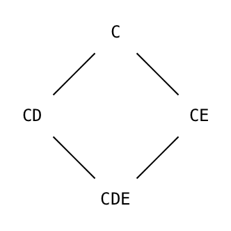
(defclass C () ())
#<STANDARD-CLASS CL-JUPYTER-USER::C>
(defclass CD (C) ())
#<STANDARD-CLASS CL-JUPYTER-USER::CD>
(defclass CE (C) ())
#<STANDARD-CLASS CL-JUPYTER-USER::CE>
(defclass CDE (CD CE) ())
#<STANDARD-CLASS CL-JUPYTER-USER::CDE>
(defmethod initialize-instance ((c c) &rest rest)
    (declare (ignore rest))
    (print "C-initialization"))
#<STANDARD-METHOD COMMON-LISP:INITIALIZE-INSTANCE (C) {10055B7993}>
(defmethod initialize-instance ((cd cd) &rest rest)
    (declare (ignore rest))
    (print "beginning CD-initialization")
    (call-next-method)
    (print "finishing CD-initialization"))
#<STANDARD-METHOD COMMON-LISP:INITIALIZE-INSTANCE (CD) {100580EFD3}>
(defmethod initialize-instance ((ce ce) &rest rest)
    (declare (ignore rest))
    (print "beginning CE-initialization")
    (call-next-method)
    (print "finishing CE-initialization"))
#<STANDARD-METHOD COMMON-LISP:INITIALIZE-INSTANCE (CE) {1005A66013}>
(defmethod initialize-instance ((cde cde) &rest rest)
    (declare (ignore rest))
    (print "beginning CDE-initialization")
    (call-next-method)
    (print "finishing CDE-initialization"))
#<STANDARD-METHOD COMMON-LISP:INITIALIZE-INSTANCE (CDE) {1005CDDA23}>
(make-instance 'C)
"C-initialization"
#<C {1005D3FE63}>
(make-instance 'CD)
"beginning CD-initialization"
"C-initialization"
"finishing CD-initialization"
#<CD {1005DA9813}>
(make-instance 'CE)
"beginning CE-initialization"
"C-initialization"
"finishing CE-initialization"
#<CE {1005E2BF93}>
(make-instance 'CDE)
"beginning CDE-initialization"
"beginning CD-initialization"
"beginning CE-initialization"
"C-initialization"
"finishing CE-initialization"
"finishing CD-initialization"
"finishing CDE-initialization"
#<CDE {1005E970C3}>
And you may also play with the auxiliary :before, :after and :around methods to order as you like the various initialization steps. As a typical example, when the essential part of the initialization work of any kenzo-object is done, then the object is finally pushed in a list which is used later as explained in the next section. This is obtained as follows.
(DEFMETHOD INITIALIZE-INSTANCE :after ((k kenzo-object) &rest rest)
           (push k *k-list*))
In this way this is done if and only if the initialization work is successfully finished, even for the more specialized structures: if for example the specialized initialization work for a simplicial set fails and stops on error, then the pushing statement concerning the weakest structure is not run.
Optimizing computations.
The Kenzo program is certainly one of the most functional programs ever written down. It is frequent that several thousands of functions are present in memory, each one being dynamically defined from other ones, which in turn are defined from other ones, and so on. In this quite original situation, the same calculations are frequently asked again. To avoid repeating these calculations, it is better to store the results and to systematically examine for each calculation whether the result is already available.
Because of this situation, it is very important not to have several copies of the same function; otherwise it is impossible for one copy to guess some calculation has already been done by another copy. This is a very important question in this program, so that the following strategy has been used. Each Kenzo object has a rigorous definition, stored as a list in the dfnt slot of the object. This is the main reason of the top class kenzo-object: making easier this process. The actual definition of the kenzo-object class:
(DEFCLASS KENZO-OBJECT ()
          ((idnm :type fixnum :reader idnm)
           (dfnt :type list :reader dfnt)
           (prpr :type list :reader prpr)
           (cmmn :type list :reader cmmn)))
This class exists only in the older version of Kenzo.
Then, when any kenzo-object is to be considered, its definition is constructed and the program firstly looks in *k-list* whether some object corresponding to this definition already exists; if yes, no kenzo-object is constructed, the already existing one is simply returned. Look at this small example where we construct the second loop space of $S^3$, then the first loop space, and then again the second loop space. In fact the initial construction of the second loop space required the first loop space, and examining the identification number K?? of these objects shows that when the first loop space is later asked for, Kenzo is able to return the already existing one.
(def s3 (sphere 3))
[K405 Simplicial-Set]
(def o2s3 (loop-space s3 2))
[K422 Simplicial-Group]
(def os3 (loop-space s3 1))
[K410 Simplicial-Group]
(def o2s3-2 (loop-space s3 2))
[K422 Simplicial-Group]
(eq o2s3 o2s3-2)
T
The last statement shows the symbols o2s3 and o2s3-2 points to the same machine address. In this way we are sure any kenzo-object has no duplicate, so that the memory process for the values of numerous functions cannot miss an already computed result. Let us look some dfnt slots:
In the newer version of Kenzo, the slot name is
orgnfor origin.
(orgn o2s3)
(LOOP-SPACE [K410 Simplicial-Group])
(orgn (k 410))
(LOOP-SPACE [K405 Simplicial-Set])
(orgn (k 405))
(SPHERE 3)
You see in this way the history of the construction process can be freely examined by the user, which is important in the development stage.
Delaying initializations.
The complete structure of a Kenzo object is extremely complicated, and many components are often useless. Another CLOS feature is therefore used to avoid the maybe non-necessary initialization works. The following artificial example explains how this is possible; it is a kind of \emph{autoloading} mechanism, elegant, easy to be used, and useful to avoid initializing needless slots. We assume a C class, where each C object has two slots, sl1 and sl2; the first one is necessary, but the second one would be the result of a complex process here simulated as being 1000 times the value of the first one.
(DEFCLASS F ()
          ((sl1 :type integer :initarg :sl1 :reader sl1)
           (sl2 :type integer :reader sl2)))
#<STANDARD-CLASS CAT:F>
(DEFMETHOD SLOT-UNBOUND (class (fi f) (slot-name (eql 'sl2)))
           (declare (ignore class))
           (setf (slot-value fi 'sl2) (* 1000 (sl1 fi)))
           (sl2 fi))
#<STANDARD-METHOD COMMON-LISP:SLOT-UNBOUND (T F (EQL SL2)) {10063DB733}>
(DEFVAR FI (make-instance 'f :sl1 23))
FI
(SLOT-BOUNDP fi 'sl2)
NIL
(sl2 fi)
23000
(SLOT-BOUNDP fi 'sl2)
T
You see the generic function slot-unbound is available which is called by the error manager when a non-initialized slot is asked for. The standard process finally does generate an error. But the user can write specialized methods for this generic function, allowing him instead to initialize the missing slot by some process using the available information. You see the initialization process lets uninitialized the sl2 slot of the F-instance located by fi, but when this slot is asked for, the "right" value is in fact returned! A new examination by slot-boundp shows the slot is now bound.
This process is extremely convenient to organize the data as a living object where each time some missing component is questionned, an automatic "repairing process" is started, computing the missing information. The process may be recursive, so that if, in the repairing process, some other datum is again missing, another repairing process is recursively started, and so on.
The following discussion (counters) applies to the older version of Kenzo.
This possibility is intensively used in the Kenzo program. Look at this small example. Firstly we reinitialize the environment by cat-init. When the fourth loop space $\Omega^4 S^5$ is constructed, you see only 26 Kenzo objects are present in the environment. Then the homology group $H_2 \Omega^4 S^5$ is asked for. The answer, $\mathbb{Z}_2$ is quickly obtained, but the number of present Kenzo objects is now 504; an enormous set of slot-unbound calls has generated the construction of 478 new Kenzo objects, necessary to do the calculation. Furthermore a :before method had been added just to count the number of slot-unbound calls, a convenient debugging trick; you see the homology calculation has recursively generated 240 slot-unbound calls.
(cat-init)
---done---
NIL
(def s5 (sphere 5))
[K1 Simplicial-Set]
(def o4s5 (loop-space s5 4))
[K42 Simplicial-Group]
(how-many-objects)
     4 SMGRs
     0 KANs
     8 SMMRs
     9 SMSTs
     0 HOPFs
     0 ALGBs
     9 CLGBs
     0 HMEQs
     0 RDCTs
    35 MRPHs
    18 CHCMs
---done---
NIL
(defparameter counter 0)
COUNTER
(defmethod slot-unbound :before (class instance slot)
    (declare (ignore class instance slot))
    (incf counter))
#<STANDARD-METHOD COMMON-LISP:SLOT-UNBOUND :BEFORE (T T T) {1006853193}>
(homology o4s5 2)
Computing boundary-matrix in dimension 2.
Rank of the source-module : 1.


;; Clock -> 2017-02-26, 2h 19m 19s.
Computing the boundary of the generator 1/1 (dimension 2) :
<<AlLp[1 <<AlLp[2 <<AlLp[3 <<AlLp[4 S5]>>]>>]>>][1 <<AlLp[2 <<AlLp[3 <<AlLp[4 S5]>>]>>]>>]>>
End of computing.


Computing boundary-matrix in dimension 3.
Rank of the source-module : 2.


;; Clock -> 2017-02-26, 2h 19m 19s.
Computing the boundary of the generator 1/2 (dimension 3) :
<<AlLp[3 <<AlLp[2 <<AlLp[3 <<AlLp[4 S5]>>]>>][2 <<AlLp[3 <<AlLp[4 S5]>>]>>]>>]>>
End of computing.


;; Clock -> 2017-02-26, 2h 19m 19s.
Computing the boundary of the generator 2/2 (dimension 3) :
<<AlLp[1 <<AlLp[2 <<AlLp[3 <<AlLp[4 S5]>>]>>]>>][1 <<AlLp[2 <<AlLp[3 <<AlLp[4 S5]>>]>>]>>][1 <<AlLp[2 <<AlLp[3 <<AlLp[4 S5]>>]>>]>>]>>
End of computing.


Homology in dimension 2 :


Component Z/2Z


---done---

;; Clock -> 2017-02-26, 2h 19m 19s.
NIL
(how-many-objects)
     4 SMGRs
     0 KANs
     8 SMMRs
    17 SMSTs
     0 HOPFs
     0 ALGBs
    17 CLGBs
    16 HMEQs
    46 RDCTs
   395 MRPHs
    90 CHCMs
---done---
NIL
counter
5
Mixing low level and high level programming.
Computing time is crucial for the applications of the Kenzo program. The complexity of the implemented algorithms is highly exponential, so that the developer must carefully consider how he can improve the computing time of the written down Lisp code. In particular, if the heart of the program may be written close to the machine language, large amounts of computing time can be saved. But conversely this must not penalize the readability and the modularity of the program.
Which is striking with the current version of Common Lisp is the possibility of easily mixing low level and high level programming. The features about OOP previously described in this paper show how Common Lisp is powerful in high level programming, allowing the user to directly handle the sophisticated objects of Algebraic Topology such as chain complexes, products and coproducts, Hopf algebras, simplicial sets and simplicial groups.
iut on the other hand, the Kenzo program intensively uses the low level part of the Common Lisp language, that is, the quasi-assembler language which is the very root of the language, such as the popular (?) car, cdr, and cons. This is possible thanks to the Common Lisp macrogenerator, already mentioned Section 3.5. Let us consider the case of the type absm, that is, abstract simplex. These objects are really the most elementary consituents of the Kenzo geometric objects, and they are so intensively used, billions of times for every sgnificant Kenzo run, that you must not use CLOS for these kernel structures. Kenzo defines the absm type as follows:
(DEFUN ABSM-P (object)
       (declare (type any object))
       (the boolean
            (and (consp object)
                 (eq :absm (car object))
                 (typep (cdr object) 'iabsm))))

(DEFTYPE ABSM () '(satisfies absm-p))
The absm-p function explains an absm is a cons (pair) where the lefthand component is the keyword :absm and the righthand one is an iabsm, that is, an internal absm; in the same way, elsewhere in the program, it is explained an iabsm is again a cons where the righthand component is anything and the lefthand component is a fixnum coding a degeneracy operator. Most of computations in Algebraic Topology are in fact low level computations about degeneracy
operators where such an operator is a decreasing list of small integers, like (5 2 0); because this list is strictly decreasing, it can be represented by the fixnum 37 because $37 = 2^5 + 2^2 + 2^0$, so that all the standard calculations about degeneracy operators become fine calculations at the bit level on binary fixnums. But Common Lisp has all the
predefined functions to do such a job, so that the programmer can efficiently work according to this strategy. A considerable memory space is saved so and furthermore the calculations are much faster.
If a degeneracy operator is to be extracted from an absm, the dgop macro is used:
(DEFMACRO DGOP (absm)
          `(the dgop (cadr (the cadr ,absm)))
which explains that in fact the call of dgop is synonymous with a call of the assembler-like cadr, but the types of argument and result are verified:
(dgop (absm 37 'something))
37
(dgop 'not-an-absm)
TYPE-ERROR:
  #<TYPE-ERROR expected-type: "ABSM"datum: NOT-AN-ABSM>
NIL
When the program is compiled, the compiler firstly translates the source code when a macro call is found, so that it is an assembler-like statement which is compiled; furthermore an appropriate compiler option allows the compiled code to ignore or not the type verifications through the (the ...) statements. When the program is finalized for production work, of course these type verifications are discarded to save computing time. You see in this way the Lisp code is readable, this code being firstly translated in low level Lisp statements, therefore very efficiently compiled, without loosing if
necessary the type verifications.
References
[CRML] Gunnar Carlsson and R. James Milgram. Stable homotopy and iterated loop spaces. in [JAMS], pp 505-583.
[DRSS] Xavier Dousson, Julio Rubio, Francis Sergeraert and Yvon Siret.The Kenzo program. Source
[JAMS] Handbook of Algebraic Topology (Edited by I.M. James). North-Holland (1995).
[KCRB] Gregor Kiczales, Jim des Rivières and Daniel G. Bobrow. The Art of the Metaobject Protocol. MIT Press, 1991.
[RBSR6] Julio Rubio, Francis Sergeraert.Constructive Algebraic Topology. Talk at the EACA Conference of Tenerife, 1999. To appear in Bulletin des Sciences Mathématiques.
[SRGR3] Francis Sergeraert.The computability problem in algebraic topology. Advances in Mathematics, 1994, vol. 104, pp 1-29.
[SRGR5] Francis Sergeraert. $\maltese_k$, objet du 3e type. Gazette des Mathématiciens, 2000, vol. 86, pp 29-45.
[STEL1] Guy L. Steele Jr. Common Lisp. Digital Press, 1984.
[STEL2] Guy L. Steele Jr. Common Lisp, second edition. Digital Press, 1990.